Assignment 10: Quantifying Investment Risk

Discussion on Monday 4/6/26
Workshop in class on Wednesday 4/8/26
Submission due by 9:00 p.m. on Friday 4/10/26.

Preliminaries

In your work on this assignment, make sure to abide by the collaboration policies of the course.

For each problem in this problem set, we will be writing or evaluating some Python code. You are encouraged to use the Spyder IDE which will be discussed/presented in class, but you are welcome to use another IDE if you choose.

If you have questions while working on this assignment, please post them on Piazza! This is the best way to get a quick response from your classmates and the course staff.

If you have questions while working on this assignment, please post them on Piazza! This is the best way to get a quick response from your classmates and the course staff.

Objective and Overview

Objective: More practice with time-series data and investment returns.

Overview: In this assignment, you will implement some functions to to help quantify the risk of an investment strategy. In particular, you will implement computations of two risk metrics: the value at risk and the drawdown of an investment.

pip3 install numpy scipy matplotlib pandas

Task 1: Quantifying Investment Risk, Part 1: Value at Risk

40 points; individual-only

Value at Risk is a measure of how much (in dollars or percentage) we expect an investment to lose if a very bad series of events occurs over a given time horizon. For example, if things go really badly, how much would we lose in 10 days?

There are many methods to calculate the value at risk, but a common approach is to assume approximately normally distributed investment returns and to construct a confidence level about how bad a loss we might sustain over a given time horizon.

Do this entire task in a file called a10task1.py.

1. Write a function compute_model_var_pct(mu, sigma, x, n) to compute the value at risk as a percentage of the asset/portfolio value.

   The function must return the value at risk as a floating point number.

   This version of the Value at Risk estimate will use a model of the asset’s returns, assuming a normal distribution of daily returns, described by the parameters mu (the mean daily rate of return) and sigma (the daily standard deviation of returns).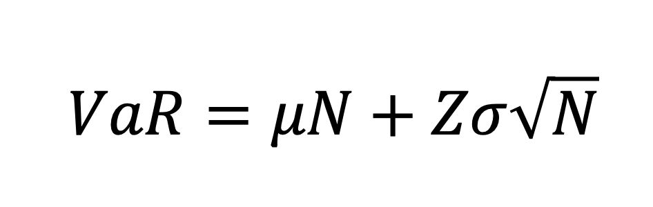

   

   The function parameters x and n are used to calibrate the estimate of VaR for the confidence level that the maximum loss during the number of days will not be exceeded. In words, we want to be x percent confident of our maximum (percentage) loss over the course of n consecutive days.

   Here is an example of using this function call:

   # estimate the 10-day VaR (98% confidence) 
   # using a mean daily return of 0.0008 and standard deviaton of 0.01
   >>> compute_model_var_pct(0.0008, 0.01, 0.98, 10)
   -0.05694524299686158
   
   # estimate the 14-day VaR (97% confidence) 
   # using a mean daily return of 0.001 and standard deviaton of 0.015
   >>> compute_model_var_pct(0.001, 0.015, 0.97, 14)
   -0.09155927945404512
   

   Note: the value Z is a quantity of standard deviations corresponding to the confidence level. Use the function scipy.stats.norm.ppf(p), where p corresponds to the probability of an event outside the confidence level, e.g. p = 1 - x.

2. Write the compute_historical_var_pct(returns, x, n), to compute the VaR (as a percentage) using the historical simulation approach.

   The function must return the value at risk as a floating point number.

   The parameter returns is a Pandas Series containing historical daily stock returns, with a date index.

   The function parameters x and n are used to calibrate the estimate of VaR for the confidence level that the maximum loss during the number of days will not be exceeded. In words, we want to be x percent confident of our maximum (percentage) loss over the course of n consecutive days.

   Procedure

   In this function, we must begin by sorting the daily returns. Use the confidence level x to find the nth worst day’s return.

   For example, suppose we have 500 daily returns and we need the 99% confidence level. We will use the rate of return from the 495th worst day, which will exclude the worst outliers. This is our one-day value at risk at the 99% confidence level.

   For a multi-day VaR calculation, we need to scale this value by the time horizon, i.e.:

   

   Example 1: Here is some example program output using data from the SPY exchange-traded fund, using 1000 daily returns:

   count    1001.000000
   mean        0.000370
   std         0.011934
   min        -0.115887
   25%        -0.002503
   50%         0.000554
   75%         0.004663
   max         0.086731
   Name: r, dtype: float64
   
   With compute_historical_var_pct estimate, we are 98% confident 
   that the maximum loss over 7 days would not exceed -7.69%.
   

   Example 2: Here is some example program output using data from the SPY exchange-traded fund, using 500 daily returns:

   count    501.000000
   mean       0.000153
   std        0.015369
   min       -0.115887
   25%       -0.003538
   50%        0.000599
   75%        0.005502
   max        0.086731
   Name: r, dtype: float64
   
   With the compute_historical_var_pct estimate, we are 99% confident 
   that the maximum loss over 10 days would not exceed -14.56%.
   

   Note that the choice of the historical data set has a substantial impact on which data values are used for the nth worst day. Your results might not match these exact values (depending on the data set you use), but they should be close.

Task 2: Quantifying Investment Risk, Part 2: Drawdown

40 points; individual-only

Drawdown is a measure of the loss of value from the most recent maximum value until today. Investors are concerned about the worst-case scenario, and drawdown helps to quantify this worst-case.

For example, here is a chart showing the daily price history (blue line) for GM shares for the calendar year 2017, as well as the previous maximum price (orange line):

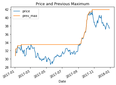
An investor who remembers the “high price” of the stock on 2017-10-24, will feel that they have lost value since that price ($41.95). The “drawdown” as of 2017-12-29 is $4.62, i.e., a loss of about 12% from that previous maximum.

Here is another graph of the same time frame, showing the drawdown in percentage terms:

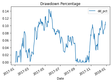
Do this entire task in a file called a10task2.py.

1. Write the function compute_drawdown(prices), which processes a column of asset prices. The parameter prices could be a np.array object (or subclass, e.g., a pandas.Series or pandas.DataFrame) containing a column array (n x 1) of asset prices, which we assume to be sequential (i.e. daily).

   The function returns a pandas.DataFrame object containing these columns:
   price, which is a copy of the data in the parameter prices
prev_max, which contains the previous peak price before this price,
   dd_dollars, which is the drawdown since the previous maximum price, measured in dollars,
   dd_pct, which is the percentage decline since the previous maximum price
   

   Here is an example of using this function, as well as the last several rows that it produces:

   >>> df = pd.read_csv('/Users/azs/Downloads/GM.csv')
   >>> # set the 'Date' column as index
   >>> df.index = pd.to_datetime(df['Date'])
   >>> prices = pd.DataFrame(df.loc['2017-01-01':'2017-12-31','Adj Close'])
   >>> # compute drawdown for this one stock
   >>> dd = compute_drawdown(prices)
   >>> dd.describe()       
               price    prev_max  dd_dollars      dd_pct
   count  251.000000  251.000000  251.000000  251.000000
   mean    33.544823   35.603981    2.059158    0.057907
   std      3.635670    3.558961    1.384220    0.038419
   min     28.647619   30.745390    0.000000    0.000000
   25%     30.741016   33.483166    0.859024    0.025709
   50%     32.214863   33.483166    2.078591    0.058816
   75%     36.899145   37.336340    3.217404    0.088337
   max     41.953167   41.953167    4.835547    0.144417
   
   >>> dd.tail(10)
               price       prev_max  dd_dollars    dd_pct
   Date                                                  
   2017-12-15  37.298019  41.953167    4.655148  0.110961
   2017-12-18  38.390999  41.953167    3.562168  0.084908
   2017-12-19  38.700676  41.953167    3.252491  0.077527
   2017-12-20  38.728004  41.953167    3.225163  0.076875
   2017-12-21  38.400105  41.953167    3.553062  0.084691
   2017-12-22  38.272587  41.953167    3.680580  0.087731
   2017-12-26  38.072212  41.953167    3.880955  0.092507
   2017-12-27  37.625912  41.953167    4.327255  0.103145
   2017-12-28  37.689667  41.953167    4.263500  0.101625
   2017-12-29  37.334450  41.953167    4.618717  0.110092
   

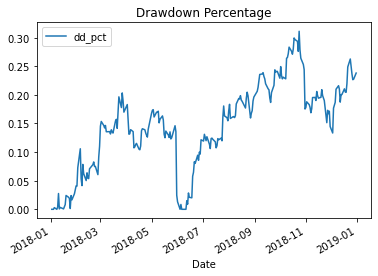
2. Write the function plot_drawdown(df), which will create and show two charts:

   1 - The historical price and previous maximum price.

   2 - The drawdown since previous maximum price as a percentage lost.

   The parameter df, is a pandas.DataFrame object containing these columns:
   price, which is a copy of the data in the parameter prices
prev_max, which contains the previous peak price before this price
   dd_dollars, which is the drawdown since the previous maximum price, measured in dollars
   dd_pct, which is the percentage decline since the previous maximum price
   

   (i.e., the same data as the results from the function compute_drawdown(prices)).

   Here is an example of using this function:

   >>> df = pd.read_csv('/Users/azs/Downloads/GM.csv')
   >>> # set the 'Date' column as index
   >>> df.index = pd.to_datetime(df['Date'])
   >>> prices = pd.DataFrame(df.loc['2008-01-01':'2008-12-31','Adj Close'])
   >>> # compute drawdown for this one stock
   >>> dd = compute_drawdown(prices)
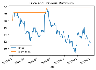
   >>> plot_drawdown(dd)
   

   The above example produces these graphs:

3. Write the function run_mc_drawdown_trials(init_price, years, r, sigma, trial_size, num_trials). This function will use the Monte Carlo stock simulation that you wrote in Assignment 8 to simulate the price path evoluation of a stock. Specifically, you will create an instance of the MCStockSimulator class, and run num_trials, and calculate the maximum drawdown for each trial.

   The parameters are: init_price: the initial stock price at time 0 of the simulation,
   years: the number of years the simulation should run
   r: the mean annual rate of return,
   sigma: the standard deviation of annual returns,
   trial_size: the number of discrete steps per year, i.e., number of trading days,
   num_trials: the number of trials to include in this simulation run.
   

   The function returns a pd.Series object of the trial results (maximum drawdown of each trial).

   To begin, you must add this import statement at the top of your file:

       from a8task1 import MCStockSimulator
   

   Note, you will need to upload the file a8task1.py with your submission.

   Here is a sample of calling this function. Note that with 100 trials of 2520 periods, this took several minutes to complete. You should begin your testing with smaller numbers, e.g., 10 trials of 12 periods, and check that everything works before increasing the running time requirements.

       >>> # Using historical AAPL prices
       >>> # Using historical AAPL prices
       >>> df = pd.read_csv('/Users/azs/Downloads/AAPL.csv')
       >>> df['ret'] = np.log(df['Adj Close'] / df['Adj Close'].shift(1))    
       >>> trial_size = 252 # trading days/year
       >>> init_price = float(df['Adj Close'].sample())
       >>> r = df['ret'].mean() * trial_size
       >>> sigma = df['ret'].std() * np.sqrt(trial_size)
       >>> years = 10
       >>> num_trials = 100
       >>> max_dd = run_mc_drawdown_trials(init_price,  years, r, sigma, trial_size, num_trials)
       >>> max_dd.describe()
       count    100.000000
       mean       0.489571
       std        0.094382
       min        0.321985
       25%        0.423104
       50%        0.482001
       75%        0.543692
       max        0.740162
       dtype: float64
       >>> max_dd.hist()
   

   The above example produces this chart:

   

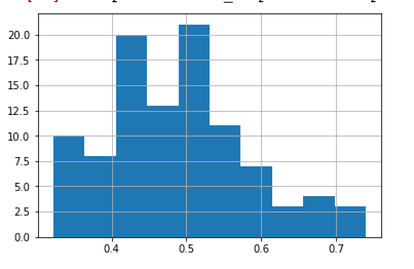
   In this graph, the possible drawdown (loss) is on the horizontal axis, and the veritcal axis shows the fraction of all trials with such a loss.

   Notes:

   • Create a new np.array to hold the results of the trials. After collecting the result, create and return a pd.Series object with these results.

   • Use an accumulator pattern to execute num_trials trials, and to caclulate the maximum drawdown for each trial.

Submitting Your Work

20 points; will be assigned by code review

Use the link to GradeScope (left) to submit your work.

Be sure to name your files correctly!

Under the heading for Assignment 10, attach these 4 required files:

`a8task1.py`,
`a10task1.py, 
`a10task1.py`, 
`a10task2.py` and 
`a10graphs.pdf`.

In addition, please upload all .csv data files used by your program.

When you upload the files, the autograder will test your functions/programs.

*   Why does this happen? When the autograder imports your file, the `print` 
    statement(s) execute (at import time), which causes this error.

*   You can prevent this error by not having any `print` statements in the global scope.
    Instead, create an `if __name__ == '__main__':` section at the bottom of the file, and
    put any test cases/print statements in that controlled block. For example:

        if __name__ == '__main__':

            ## put test cases here:
            print('fv_lump_sum(0.05, 2, 100)', fv_lump_sum(0.05, 2, 100))

*   `print` statements inside of functions do not cause this problem.

Notes:

• You may resubmit multiple times, but only the last submission will be graded.