Assignment 2: Bonds and Bond Math
Discussion on Monday 1/26/26
Workshop in class on Wednesday 1/28/26
Submission due by 9:00 p.m. on Friday 1/30/26.
Preliminaries
In your work on this assignment, make sure to abide by the collaboration policies of the course.
For each problem in this problem set, we will be writing or evaluating some Python code. You are encouraged to use the Spyder IDE which will be discussed/presented in class, but you are welcome to use another IDE if you choose.
If you have questions while working on this assignment, please post them on Piazza! This is the best way to get a quick response from your classmates and the course staff.
Programming Guidelines
-
Refer to the class Coding Standards for important style guidelines. The grader will be awarding/deducting points for writing code that comforms to these standards.
-
Every program file must begin with a descriptive header comment that includes your name, username/BU email, and a brief description of the work contained in the file.
-
Every function must include a descriptive docstring that explains what the function does and identifies/defines each of the parameters to the function.
-
Your functions must have the exact names specified below, or we won’t be able to test them. Note in particular that the case of the letters matters (all of them should be lowercase), and that some of the names include an underscore character (
_). -
Make sure that your functions return the specified value, rather than printing it. None of these functions should use a
printstatement. -
If a function takes more than one input, you must keep the inputs in the order that we have specified.
-
You should not use any Python features that we have not discussed in class or read about in the textbook.
-
Your functions do not need to handle bad inputs – inputs with a type or value that doesn’t correspond to the description of the inputs provided in the problem.
-
You must test each function after you write it. Here are two ways to do so:
-
Run your
a2task1.pyfile after you finish a given function. Doing so will load your latest code into the shell, where you can call the function using different inputs and check to see that you obtain the correct outputs. -
Add test calls to the bottom of your
a2task1.pyfile. These will be called every time that you run the file, which will save you from having to enter the tests yourself. We have given you an example of one such test in the starter file.
-
Warnings: Individual Work, Generative AI, and Academic Conduct!!
-
This is an individual assignment. You may discuss the problem statement/requirements, Python syntax, test cases, and error messages with your classmates. However, each student must write their own code without copying or referring to other student’s work.
-
It is strictly forbidden to use any code that you find from online websites including but not limited to as CourseHero, Chegg, or any other sites that publish homework solutions.
-
It is strictly forbidden to use any generative AI (e.g., ChatGPT, Claude, Gemini, CoPilot or any similar tools**) to write solutions for any assignment.
Students who submit work that is not authentically their own individual work will earn a grade of 0 on this assignment and a reprimand from the office of the Dean.
If you have questions while working on this assignment, please post them on Piazza! This is the best way to get a quick response from your classmates and the course staff.
Task 1: Discounted Cashflows and Bond Pricing
30 points; individual-only
Do this entire task in a file called a2task1.py.
-
Write the function
cashflow_times(n, m)to develop the list of the times at which a bond makes coupon payments, withnyears andmcoupon payments per year.For example:
>>> cashflow_times(5,2) # 5-year bond with 2 coupons/year
[1, 2, 3, 4, 5, 6, 7, 8, 9, 10]
>>> cashflow_times(3,4) # 3-year bond with 4 coupons/year
[1, 2, 3, 4, 5, 6, 7, 8, 9, 10, 11, 12]
>>> cashflow_times(2,12) # 2-year bond with monthly coupons
[1, 2, 3, 4, 5, 6, 7, 8, 9, 10, 11, 12, 13, 14, 15, 16, 17, 18, 19, 20, 21, 22, 23, 24]
>>>
Notes:
- Your function must use a list comprehension (no loops or recursion),
and requires no
if-elif-elselogic.
- Your function must use a list comprehension (no loops or recursion),
and requires no
-
Write the function
discount_factors(r, n, m)to calculate and return a list of discount factors for a given annualized interest rater, fornyears, andmdiscounting periods per year.Your function must use a list comprehension (no loops or recursion).

For example:
>>> # 3% rate, 1 years, 2 payments/year
>>> discount_factors(0.03, 1, 2)
[0.9852216748768474, 0.9706617486471405]
>>> # 5% rate, 5 years, 2 payments/year
>>> discount_factors(0.05, 5, 2)
[0.9756097560975611, 0.9518143961927424, 0.928599410919749, 0.9059506447997552, 0.8838542876095173, 0.8622968659605048, 0.8412652350834192, 0.8207465708130922, 0.8007283617688704, 0.7811984017257273]
Notes:
-
Your function must use a list comprehension (no loops or recursion), and requires no
if-elif-elselogic. -
You may assume that
mandnare integers.
-
-
Write the function
bond_cashflows(fv, c, n, m)to calculate and return a list of cashflows for a bond specified by the parameters. The parameters are:fvis the future (maturity) value of the bond;
cis the annual coupon rate expressed as percentage per year;
nis the number of years until maturity;
mis the number of coupon payments per year.In general, the coupon payment is given by:

The final payment of the bond is a coupon payment plus the maturity value (fv) of the bond.
For example:
>>> bond_cashflows(1000, 0.08, 5, 2) # 5 year bond with 2 coupons/year
[40.0, 40.0, 40.0, 40.0, 40.0, 40.0, 40.0, 40.0, 40.0, 1040.0]
>>> bond_cashflows(10000, 0.0575, 2, 2) # 2 year bond with 2 coupons/year
[287.5, 287.5, 287.5, 10287.5]
>>> bond_cashflows(5000, 0.09, 2, 4) # 2 year bond with 4 coupons/year
[112.5, 112.5, 112.5, 112.5, 112.5, 112.5, 112.5, 5112.5]
Notes:
-
Your function must use a list comprehension (no loops or recursion), and requires no
if-elif-elselogic. -
Re-use your
cashflow_times(n, m)function to obtain the list of the times of the cashflows for this bond – this will give you the correct number of cashflows. -
Notice that the last period’s casflow includes the maturity vale (
fv) of the bond as well as the last coupon payment.
-
-
Write the function
bond_price(fv, c, n, m, r)to calculate and return the price of a bond. The parameters are:fvis the future (maturity) value of the bond;
cis the annual coupon rate expressed as percentage per year;
nis the number of years until maturity;
mis the number of coupon payments per year;
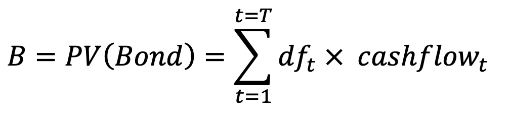
andr, the annualized yield to maturity of the bondThe price of the bond B is the sum of the present values of the cashflows of that bond:
For example:
>>> # 3-year, 4% coupon bond, semi-annual coupons, priced at 4% annualized YTM.
>>> bond_price(100, 0.04, 3, 2, 0.04)
100.0 # sells at par
>>> # 3-year, 4% coupon bond, semi-annual coupons, priced at 3% annualized YTM.
>>> bond_price(100, 0.04, 3, 2, 0.03)
102.84859358273769 # sells at a premium
>>> # 3-year, 4% coupon bond, semi-annual coupons, priced at 5% annualized YTM.
>>> bond_price(100, 0.04, 3, 2, 0.05)
97.24593731921014 # sells at a discount
Important Implementation Notes:
-
Your function must use a list comprehension (no loop with an accumulator pattern or recursion) and requires no
if-elif-elselogic. Consider the equation above, and how you could use a list comprehension to build this result. -
Re-use your
cashflow_times(n,m)function from above to find the cashflow times for this bond. -
Re-use your
bond_cashflows(fv, c, n,m)function from above to find the cashflows associated with this bond. -
Re-use your
discount_factors(r, n, m)function from above to calculate the relevant discount factors.
-
-
Write the function
bond_yield_to_maturity(fv, c, n, m, price):to calculate the annualized yield_to_maturity on a bond. The parameters are:fvis the future (maturity) value of the bond;
cis the annual coupon rate expressed as percentage per year;
nis the number of years until maturity;
mis the number of coupon payments per year;
andpriceis the current market price of the bondRead the notes and hints before you begin to write any code*
For example, consider a 3-year bond with a 4% coupon rate, with coupons paid semi-annually. We observe the bond is selling for $101.75. The yield to maturity is the implied interest rate for this bond, in this case is 3.38% per year:
>>> bond_yield_to_maturity(100, 0.04, 3, 2, 101.75)
0.03381660580635071
As a second example, consider a 5-year bond with an 8% coupon rate, with coupons paid annually. We observe the bond is selling for $950. The yield to maturity is the implied interest rate for this bond, in this case 9.29% per year:
>>> bond_yield_to_maturity(1000, 0.08, 5, 1, 950)
0.09295327519066632
This function will (in its final form) use a
whileloop to find the appropriate yield by iteration, i.e., trying many values (for the yield) until the correct yield is found (within an acceptable margin of error).Hints:
-
When you first write your function, it will be helpful to work with a definite loop (i.e., a
forloop). Make it run 10 times, and watch what happens to the interest rate and the bond price. Is it going in the right direction or not? -
Include a print statement inside your loop to show the test interest rate and the value of the bond at each iteration of the loop. For example:
>>> bond_yield_to_maturity(100, 0.04, 3, 2, 101.75)
Iteration 0, test_rate = 0.50000000, price = $32.117248 diff = $-69.632752
Iteration 1, test_rate = 0.25000000, price = $57.434695 diff = $-44.315305
Iteration 2, test_rate = 0.12500000, price = $79.264523 diff = $-22.485477
Iteration 3, test_rate = 0.06250000, price = $93.930828 diff = $-7.819172
Iteration 4, test_rate = 0.03125000, price = $102.487223 diff = $0.737223
Iteration 5, test_rate = 0.04687500, price = $98.096648 diff = $-3.653352
Iteration 6, test_rate = 0.03906250, price = $100.262983 diff = $-1.487017
Iteration 7, test_rate = 0.03515625, price = $101.367754 diff = $-0.382246
Iteration 8, test_rate = 0.03320312, price = $101.925637 diff = $0.175637
Iteration 9, test_rate = 0.03417969, price = $101.646235 diff = $-0.103765
Iteration 10, test_rate = 0.03369141, price = $101.785821 diff = $0.035821
Iteration 11, test_rate = 0.03393555, price = $101.715999 diff = $-0.034001
Iteration 12, test_rate = 0.03381348, price = $101.750903 diff = $0.000903
Iteration 13, test_rate = 0.03387451, price = $101.733449 diff = $-0.016551
Iteration 14, test_rate = 0.03384399, price = $101.742175 diff = $-0.007825
Iteration 15, test_rate = 0.03382874, price = $101.746539 diff = $-0.003461
Iteration 16, test_rate = 0.03382111, price = $101.748721 diff = $-0.001279
Iteration 17, test_rate = 0.03381729, price = $101.749812 diff = $-0.000188
Iteration 18, test_rate = 0.03381538, price = $101.750357 diff = $0.000357
Iteration 19, test_rate = 0.03381634, price = $101.750084 diff = $0.000084
Iteration 20, test_rate = 0.03381681, price = $101.749948 diff = $-0.000052
Iteration 21, test_rate = 0.03381658, price = $101.750016 diff = $0.000016
Iteration 22, test_rate = 0.03381670, price = $101.749982 diff = $-0.000018
Iteration 23, test_rate = 0.03381664, price = $101.749999 diff = $-0.000001
0.03381660580635071
This will help you verify that your algorithm is working correctly.
Remove the print statement when you are done.
Notes:
-
Review to the example from class in which we continue a guessing game until we find a solution. Create variables for the upper and lower bounds for the interest rate and use the average of these as a test rate.
Calculate the bond price using the test rate.
If the calculated price is too low, you will need to try a lower rate (which will lead to a higher price). Thus, you will need to change the upper bound to make it lower – by setting the upper bound to be the previous the test rate (which was the mid-point) from the last guess.
If the calculated price is too high, you will need to try a higher rate ...Then try again...
-
You should continue your iteration until the calculated bond price is close enough to the actual bond price, i.e., within an acceptable margin of error. Declare a variable to hold the required degree of accuracy, i.e.,
ACCURACY = 0.0001 # iterate until the error is less than $0.0001
and continue iterating until the basolute value of the difference in bond price is less than this amount of accuracy. Note: the example above uses an accuracy of 0.001, so your results will differ.
-
The yield to maturity is usually a positive number. However, there have been times where the yield on bonds (especially inflation-protected bonds) havs been negative. Make sure your function will work even with a negative yield to maturity. Test it by using a high bond price and short maturity (e.g., 1-year bond with price of $1100).
-
Task 2: Estimating the Change in Bond Price
30 points; individual-only
Interest rates and bond prices move in opposite directions. When interest rates increase, the price of a bond will decrease; when interest rates decrease, the price of a bond will increase. How much will the price of the bond increase or decrease, as a result of a change interest rates? This is an important question, to help us understand the riskiness of our bond or bond portfoio.
This graph illustrates the bond price as a function of the current yield:
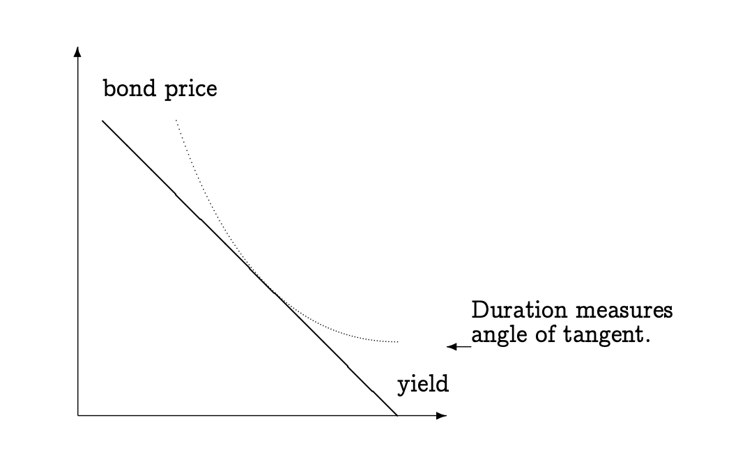
The metrics that will help us measure the sensitivity of the price of a bond to the change in interest rates are called duration and convexity, and you will compute them in this part of the assignment.
Do this entire task in a file called a2task2.py. You will need to import your work
from Task 2 to complete and test this part. Add this import statement to the top of
your a2task2.py file:
from a2task1 import *
Note: if you have any unit-test code (i.e., function calls or print statements
that are in the global scope in your a2task1.py file), those statements will run
when you import the file. One way to leave that unit test code in place, but prevent
it from running when you import the file is to put the unit test code in a special
block at the bottom of your a2task1.py file, like this:
######################################################################
### unit test code:
if __name__ == '__main__':

    times = cashflow_times(5,2)
    cashflows = bond_cashflows(100,0.04,5,2)
    df = discount_factors(0.02, 5, 2)
    price = bond_price(100, 0.04, 3, 2, 0.03)
    ytm = bond_yield_to_maturity(1000, 0.08, 5, 1, 950)


## end of unit test code
The expression __name__ == '__main__' will evaluate to True only when you run
the file, but not when the file is imported.
-
The duration of a bond is a metric that helps us estimate the sensitivity of a bond’s price to changes in the interest rate. A bond’s duration is sometimes referred to as the average maturity or the effective maturity.
The longer the duration, the longer is the average maturity, and, therefore, the greater the sensitivity to interest rate changes (i.e., duration is the 1st derivative of the price-yield curve).
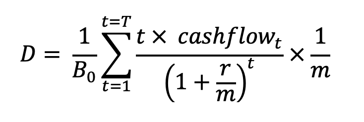
The duration is a weighted-average of the times at which each cashflow is received, and the weights are the present-values of each cashflow:
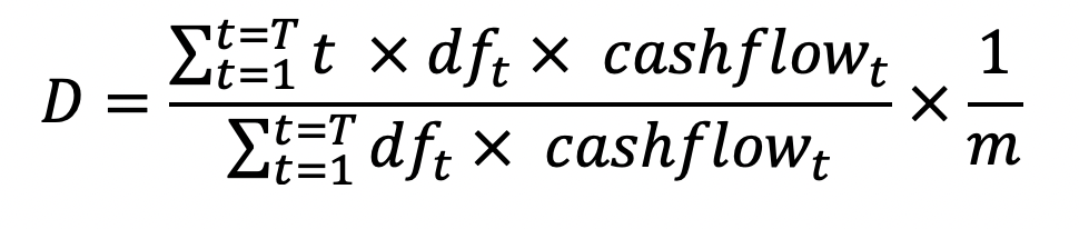
which simplifies to
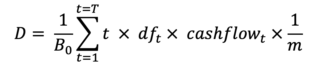
which simplifies to
Write the function
bond_duration(fv, c, n, m, r)to calculate and return the duration metric for a bond. The parameters are:fvis the future (maturity) value of the bond;
cis the annual coupon rate expressed as percentage per year;
nis the number of years until maturity;
mis the number of coupon payments per year;
andris the interest rate of the bondFor example:
>>> # example with normal (coupon) bond
>>> # 5 year bond with 2 coupons/year, fv = 1000, coupon rate = 8%, r = 7% per year
>>> bond_duration(1000, 0.08, 5, 2, 0.07)
4.2362
All other things being equal, a bond with higher coupon payments will have lower duration than a bond with lower coupon payments.
>>> # another example with normal (coupon) bond
>>> # 5 year bond with 2 coupons/year, fv = 1000, coupon rate = 14%, r = 7% per year
>>> bond_duration(1000, 0.14, 5, 2, 0.07)
3.921591061881657
And a zero-coupon bond (which pays only the maturity value in the future) will have a duration equal to its maturity:
>>> # example with a zero-coupon bond:
>>> # 5 year bond with 2 coupons/year, fv = 1000, coupon rate = 0%, r = 7% per year
>>> bond_duration(1000, 0, 5, 2, 0.07)
5.0
Notes:
-
The above examples are calculating the annualized duration, i.e., the duration per payment period multiplied by the number of payment periods. For example, a duration of 10 half-years is equal to 5 years.
-
Your function may use either a list comprehension or a definite (
for) loop with an accumulator pattern (nowhileloops or recursion) and requires noif-elif-elselogic. -
Re-use your
cashflow_times,bond_cashflows,discount_factors, andbond_pricefunctions from above as needed.
For example:
>>> # example with normal (coupon) bond selling at par
>>> # 5 year bond with 2 coupons/year, fv = 1000, coupon rate = 8%, r = 8% per year
>>> bond_duration(1000, 0.08, 5, 2, 0.08)
4.217665805264614
All other things being equal, a bond with higher coupon payments will have lower duration.
>>> # another example with normal (coupon) bond at par
>>> # 5 year bond with 2 coupons/year, fv = 1000, coupon rate = 8%, r = 8% per year
>>> bond_duration(1000, 0.12, 5, 2, 0.12)
3.9008461372497893
All other things being equal, a bond with a longer time to maturity will have a higher duration than a similar bond with shorter maturity.
>>> # another example with normal (coupon) bond at par
>>> # 10 year bond with 2 coupons/year, fv = 1000, coupon rate = 12%, r = 8% per year
>>> bond_duration(1000, 0.12, 10, 2, 0.12)
6.079058245839585
And a zero-coupon bond (which pays only the maturity value in the future) will have a duration equal to its maturity:
>>> # example with a zero-coupon bond:
>>> # 5 year bond with 2 coupons/year, fv = 1000, coupon rate = 0%, r = 8% per year
>>> bond_duration(1000, 0, 5, 2, 0.08)
5.0
-
-
A bond’s Macaulay duration is the duration, given the yield to maturity implied by the bond’s current market price.
The Macaulay duration is calculated as:
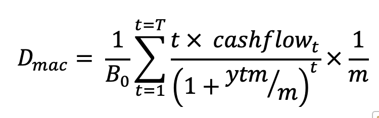
Notice that we are using the
ytmin this calculation, which we obtain by knowning the bond’s characteristics (maturity value, coupon rate, number of payments/year) and it’s current price.Write the function
macaulay_duration(fv, c, n, m, price)to calculate and return the Macaulay duration for a bond. The parameters are:fvis the future (maturity) value of the bond;
cis the annual coupon rate expressed as percentage per year;
nis the number of years until maturity;
mis the number of coupon payments per year;
andpriceis the current market price of the bond.For example:
>>> # example with normal (coupon) bond, selling at a discount
>>> # 5 year bond with 2 coupons/year, fv = 1000, coupon rate = 8%, priced at $950
>>> macaulay_duration(1000, 0.08, 5, 2, 950)
4.193711809958176
All other things being equal, a premium bond will have a higher Macaulay duration:
>>> # another example with normal (coupon) bond, selling at a premium
>>> # 5 year bond with 2 coupons/year, fv = 1000, coupon rate = 8%, priced at $1050
>>> macaulay_duration(1000, 0.08, 5, 2, 1050)
4.239752680750421
All other things being equal, a bond with a longer time to maturity will have a higher Macaulay duration than a similar bond with shorter maturity.
>>> # another example with normal (coupon) bond, selling at a premium
>>> # 10 year bond with 2 coupons/year, fv = 1000, coupon rate = 12%, priced at $1050
>>> macaulay_duration(1000, 0.12, 10, 2, 1050)
6.176862539228174
And a zero-coupon bond (which pays only the maturity value in the future) will have a Macaulay duration equal to its maturity:
>>> # example with a zero-coupon bond:
>>> # 5 year bond with 2 coupons/year, fv = 1000, coupon rate = 0%, r = 8% per year
>>> macaulay_duration(1000, 0, 5, 2, 950)
5.0
Notes:
- You may re-use your
cashflow_times,bond_cashflows,discount_factors,bond_price, andyield_to_maturityfunctions from task 1 as needed.
- You may re-use your
-
A bond’s modified duration helps us to estimate the percentage change in the value of a bond in response to a one percentage change in the yield.
The modified duration is calculated as:
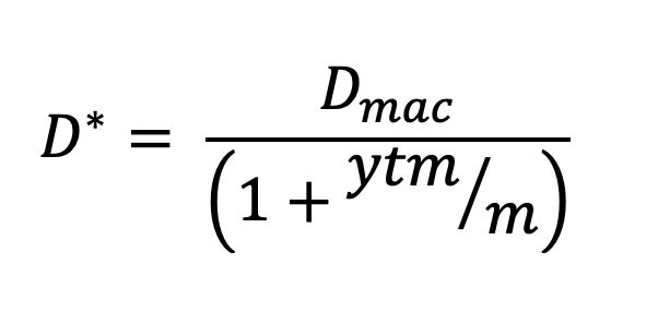
Notice that we are using the
ytmin this calculation, which we obtain by knowning the bond’s characteristics (maturity value, coupon rate, number of payments/year) and it’s current price.Write the function
modified_duration(fv, c, n, m, price)to calculate and return the Macaulay duration for a bond. The parameters are:fvis the future (maturity) value of the bond;
cis the annual coupon rate expressed as percentage per year;
nis the number of years until maturity;
mis the number of coupon payments per year;
andpriceis the current market price of the bond.For example:
>>> # example with normal (coupon) bond, selling at a discount
>>> # 5 year bond with 2 coupons/year, fv = 1000, coupon rate = 8%, priced at $950
>>> modified_duration(1000, 0.08, 5, 2, 950)
4.007900319350022
All other things being equal, increasing the number of compounding periods per year will result in a higher modified duration:
>>> # another example with normal (coupon) bond, selling at a discount
>>> # 5 year bond with 12 coupons/year, fv = 1000, coupon rate = 8%, priced at $950
>>> modified_duration(1000, 0.08, 5, 12, 950)
4.0780972745554696
>>> # 5 year bond with 365 coupons/year, fv = 1000, coupon rate = 8%, priced at $950
>>> modified_duration(1000, 0.08, 5,365, 950)
4.0920066122067125
And a zero-coupon bond (which pays only the maturity value in the future) will have a Macaulay duration equal to its maturity:
>>> # example with a zero-coupon bond:
>>> # 5 year bond with 2 coupons/year, fv = 1000, coupon rate = 0%, priced at $950
>>> modified_duration(1000, 0.0, 5, 365*24, 950)
5.0
Notes:
- You may re-use your
cashflow_times,bond_cashflows,discount_factors,bond_price, andyield_to_maturityfunctions from task 1 as needed.
- You may re-use your
-
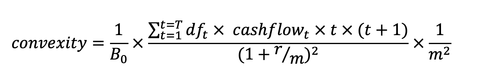
A bond’s convexity helps us improve our estimate of the bond’s price sensitivity
to changes in interest rates. Convexity describes the rate of the change in duration* as the yield changes (i.e., convexity is the 2nd derivative of the price-yield curve at the current price-yield point).Here is a formula to solve for the annualized convexity of a bond:
Notes:
-
B is the bond price (i.e., its present value). Re-use your
bond_pricefunction to find the price. -
We are calculating the annualized convexity.
Write the function
bond_convexity(fv, c, n, m, r)to calculate and return the convexity metric for a bond. The parameters are:fvis the future (maturity) value of the bond;
cis the annual coupon rate expressed as percentage per year;
nis the number of years until maturity;
mis the number of coupon payments per year;
andris the annualized yield to maturity the bondHere are some numerical examples:
>>> # example with normal (coupon) bond
>>> # $5000 pv, 0.05 coupon rate, 3 year, 2 payments/year, 5% ytm
>>> bond_price(5000, 0.05, 3, 2, 0.05)
5000.000000000003
>>> bond_duration(5000, 0.05, 3, 2, 0.05)
2.8229142478096616
>>> bond_convexity(5000, 0.05, 3, 2, 0.05)
9.210679021586303
>>>
>>> # example with a zero-coupon: 3 year bond, 2 periods/year, 5% ytm
>>> bond_duration(1000, 0, 3, 2, 0.05)
3.000000000000004
>>> bond_convexity(1000, 0, 3, 2, 0.05)
9.994051160023796
>>>
>>> # a 6-year 6.1% coupon bond, selling at a deep discount (10% ytm)
>>> bond_price(1000,0.061, 6,2, 0.10)
827.166593089248
>>> bond_duration(1000,0.061, 6,2, 0.10)
5.006797820063039
>>> bond_convexity(1000,0.061, 6,2, 0.10)
27.719199338711825
Notes:
-
The above examples are calculating the annualized duration and convexity.
-
Your
bond_convexityfunction may use either a list comprehension or a definite (for) loop with an accumulator pattern (nowhileloops or recursion) and requires noif-elif-elselogic. -
You may re-use your
cashflow_times,bond_cashflows,discount_factors, andbond_pricefunctions from task 1 as needed.
-
-
Write a function
estimate_change_in_price1(fv, c, n, m, price, dr), which will return the estimated dollar change in price corresponding to a change in yield.The parameters describe a bond by its maturity value (
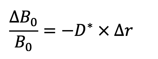
fv), coupon rate (c), years until maturity (n), the number of payments per year (m), the current bond price (price), and the change in interest rate (dr) we are modeling.In this “first approximation”, we will estimate the change in price by using the bond’s modified duration:
Notes:
-
B is the bond price (i.e., its present value). Re-use your
yield_to_maturityfunction to find the appropriateytmfor this bond price. -
D* is the modified duration of the bond at it’s current yield-to-maturity.
-
∆r is the change in interest rate from the current
ytm -
This equation is solving for the change in bond price. Your function must return the dollar-value of that change.
Example with a 1-basis point (0.0001) change in yield:
>>> # Estimate of change in price for a 5-year 7.00% coupon bond
>>> # at a current ytm of 7.00% per year:
>>> orig_price = bond_price(1000, 0.07, 5, 2, 0.07)
>>> orig_price
1000.00
>>>
>>> # what happens to bond price when the rate changes by 0.0001 (+0.01%)?
>>> dr = 0.0001
>>> est1 = estimate_change_in_price1(1000, 0.07, 5, 2, 1000, dr)
>>> est1
-0.42 # bond price estimated to decrease by $0.42
>>>
>>> new_price = bond_price(1000, 0.07, 5, 2, 0.07+dr)
>>> new_price
999.58
>>> # how close was our estimate?
>>> diff = new_price - old_price - est1
>>> diff
0 # pretty good!
Another example, with a 100-basis point (0.01) change in yield:
>>> # Estimate of change in price for a 5-year 7.00% coupon bond
>>> # at a current ytm of 7.00% per year:
>>> orig_price = bond_price(1000, 0.07, 5, 2, 0.07)
>>> orig_price
1000.00
>>>
>>> # what happens to bond price when the rate changes by 0.01 (+1%)?
>>> dr = 0.01
>>> est1 = estimate_change_in_price1(1000, 0.07, 5, 2, 1000, dr)
>>> est1
-41.58 # bond price estimated to decrease by $41.58
>>>
>>> new_price = bond_price(1000, 0.07, 5, 2, 0.07+dr)
>>> new_price
959.45
>>> # how close was our estimate?
>>> diff = new_price - old_price - est1
>>> diff
1.03 # not that close for a 1% change in yield
-
-
Write a function
estimate_change_in_price2(fv, c, n, m, price, dr), which will return the estimated dollar change in price corresponding to a change in yield.The parameters describe a bond by its maturity value (
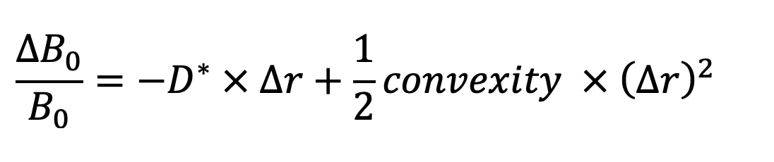
fv), coupon rate (c), years until maturity (n), the number of payments per year (m), the current bond price (price), and the change in interest rate (dr) we are modeling.In this estimate, we will improve upon the “first approximation” (duration only) by add a second term to account for the convexity of the price-yield curve.
Notes:
-
B is the bond price (i.e., its present value). Re-use your
yield_to_maturityfunction to find the appropriateytmfor this bond price. -
D* is the modified duration of the bond at it’s current yield-to-maturity.
-
∆r is the change in interest rate from the current
ytm -
This equation is solving for the change in bond price. Your function must return the dollar-value of that change.
Example, with a 100-basis point (0.01) decrease in yield:
>>> # Estimate of change in price for a 5-year 7.00% coupon bond
>>> # at a current ytm of 7.00% per year:
>>> orig_price = bond_price(1000, 0.07, 5, 2, 0.07)
>>> orig_price
1000.00
>>>
>>> # what happens to bond price when the rate changes by 0.01 (+1%)?
>>> dr = -0.01
>>> est2 = estimate_change_in_price2(1000, 0.07, 5, 2, 1000, dr)
>>> est2
42.63098958653342 # bond price estimated to increase by $41.58
>>>
>>> new_price = bond_price(1000, 0.07, 5, 2, 0.07+dr)
>>> new_price
1042.651014183879
>>> # how close was our estimate?
>>> diff = new_price - orig_price - est2
>>> diff
0.020024597344843187 # pretty close, even for a 1% change in yield
-
Task 3: Simulating a Bond Auction
20 points; individual-only
The US Treasury sells new bonds to investors by offering an auction. Interested investors must submit their bids in advance of a deadline, and the Treasury sells the bonds to investors at the highest possible prices (i.e., lowest yield to maturity) and thus the least interest cost.
The auction announcement specifies the type of security to be sold (e.g., 5-year bonds with a 3% annual coupon rate), and the amount the Treasury is planning to sell (e.g., $500,000 of maturity value). The potential investors bids must specify the price they are willing to pay per $100 of maturity value (e.g., paying $99.50 per $100 bond in this example would give an annualized yield-to-maturity of about 3.1088%).
In this task, you will write some functions to create a simple bond auction. To begin,
you should download this sample.csv file containing a list of
investor’s bids. You will process this file to determine which bids will be accepted
(i.e., those with the highest prices), and the minimum price that is successful in the
auction. The design you should follow includes 3 functions, described below.
You may write additional helper function if you find that useful, but they will not be
graded. Do this entire task in a file called a2task3.py.
Video Example: Processing a CSV data file.
Here is a video example that demonstrates how to read a file in Python, and how
to process a .CSV data file using a for loop and list indexing.
Video Example: Formatting Numeric Output.
Here is a video example that demonstrates how to produce beautifully-formatted numeric outputs.
-
Write the function
collect_bids(filename)to process the data file containing the bids. The data file will be in this format:bid_id, bid_amount, bid_price 1, 100000, 101.50 2, 100000, 101.25 3, 200000, 100.75
in which the first row contains the column headers, and each additional row contains three fields: the
bid_idwhich identifies the bidder, thebid_amount(dollar value) of bonds the this investor would like to buy, and thebid_pricethat the investor is willing to pay.Your task in this function is to process the file and return a list containing the bids (i.e., a list of lists). For example:
For example:
>>> # call the function
>>> bids = collect_bids('./bond_bids.csv')
>>> print(bids) # show the data that was returned
[[1, 100000, 101.5],
 [2, 100000, 101.25],
 [3, 200000, 100.75],
 # ...]
-
Write the function
print_bids(bids)to process the a of bids, and produce a beautifully-formatted table of the bids. In your function, you will process a list containing bids one line at a time.For each bid (a list of 3 fields), you will separate the fields into separate variables and print with appropriate formatting, i.e., with dollar signs, clean spacing, nicely lined up, etc. For example:
>>> bids = collect_bids('./bond_bids.csv')
>>> print_bids(bids)
  Bid ID          Bid Amount           Price
       1        $      100000   $     101.500
       2        $      100000   $     101.250
       3        $      200000   $     100.750
-
Write the function
find_winning_bids(bids, total_offering_fv, c, n, m)that processes a list ofbidsand determine which are successful in the auction. The parameters are:
bids, where each bid is a sublist in the form of[bid_id, bid_amount, bid_price],
total_offering_fvis the total amount of bonds being sold,
cis the annualized coupon rate,
nis the number of years to maturity for the bonds, and
mis the number of coupon payments per year.The function must do the following tasks:
-
sort the bids by
bid_price(in descending order), followed bybid_amount(in descending order). That is, the auction will give preference to the highest bidder, and if there is a tie for onebid_price, thebid_amountwill be used to break the tie. -
determine which bids will be accepted, including any partial amounts filled.
-
find the auction’s
clearing_price, which is lowest price at which the auction amount (total_offering_fv) is sold out. -
print out the table showing all bids and the amount sold to each bidder. The amount sold might be the full
bid_amount’, a fractionbid_amountif the entire bid was not filled, or0if the bid was unsuccessful. -
print out the auction clearing bond price (i.e., the price at which the offering sells out) and the yield to maturity.
-
return the list of bids, with the actual amonut sold to each bidder.
Example 1:
This test code:
if __name__ == '__main__':

    # read in the bids
    bids = collect_bids('./bond_bids.csv')
    print("Here are all the bids:")
    print_bids(bids)
    print()

    # process the bids in an auction of $500,000 of 5-year 3% semi-annual coupon bonds
    processed_bids = find_winning_bids(bids, 500000, 0.03, 5, 2)
Produces this output:
Here are all the bids:
  Bid ID          Bid Amount           Price
       1        $      100000   $     101.500
       2        $      100000   $     101.250
       3        $      200000   $     100.750
       4        $      400000   $     101.200
       5        $      250000   $     100.900
       6        $      300000   $     100.700
       7        $      120000   $     101.000
       8        $      150000   $     101.200
       9        $      100000   $     101.750
      10        $      350000   $     100.500

Here are all of the bids, sorted by price descending:
  Bid ID          Bid Amount           Price
       9        $      100000   $     101.750
       1        $      100000   $     101.500
       2        $      100000   $     101.250
       4        $      400000   $     101.200
       8        $      150000   $     101.200
       7        $      120000   $     101.000
       5        $      250000   $     100.900
       3        $      200000   $     100.750
       6        $      300000   $     100.700
      10        $      350000   $     100.500

The auction is for $500000.00 of bonds.

4 bids were successful in the auction.
The auction clearing price was $101.200, i.e., YTM is 0.027415 per year.
Here are the results for all bids:

  Bid ID          Bid Amount           Price
       9        $      100000   $     101.750
       1        $      100000   $     101.500
       2        $      100000   $     101.250
       4        $      200000   $     101.200
       8        $           0   $     101.200
       7        $           0   $     101.000
       5        $           0   $     100.900
       3        $           0   $     100.750
       6        $           0   $     100.700
Example 2:
This test code:
if __name__ == '__main__':

    # read in the bids
    bids = collect_bids('./bond_bids.csv')
    print("Here are all the bids:")
    print_bids(bids)
    print()

    # process the bids in an auction of $1,400,000 of 5-year 3.25% semi-annual coupon bonds
    processed_bids = find_winning_bids(bids, 1400000, 0.0325, 5, 2)
Produces this output:
Here are all the bids:
  Bid ID          Bid Amount           Price
       1        $      100000   $     101.500
       2        $      100000   $     101.250
       3        $      200000   $     100.750
       4        $      400000   $     101.200
       5        $      250000   $     100.900
       6        $      300000   $     100.700
       7        $      120000   $     101.000
       8        $      150000   $     101.200
       9        $      100000   $     101.750
      10        $      350000   $     100.500

Here are all of the bids, sorted by price descending:
  Bid ID          Bid Amount           Price
       9        $      100000   $     101.750
       1        $      100000   $     101.500
       2        $      100000   $     101.250
       4        $      400000   $     101.200
       8        $      150000   $     101.200
       7        $      120000   $     101.000
       5        $      250000   $     100.900
       3        $      200000   $     100.750
       6        $      300000   $     100.700
      10        $      350000   $     100.500

The auction is for $1400000.00 of bonds.

8 bids were successful in the auction.
The auction clearing price was $100.750, i.e., YTM is 0.030870 per year.
Here are the results for all bids:

  Bid ID          Bid Amount           Price
       9        $      100000   $     101.750
       1        $      100000   $     101.500
       2        $      100000   $     101.250
       4        $      400000   $     101.200
       8        $      150000   $     101.200
       7        $      120000   $     101.000
       5        $      250000   $     100.900
       3        $      180000   $     100.750
       6        $           0   $     100.700
      10        $           0   $     100.500
Implementation Notes:
-
To sort the bids by price, use the technique that was shown in class with a list comprehension and a list-of-lists. Once you have the appropriate list-of-lists, you can use the built-in
listsorting method calledsort(). For example, experiment with this code at the Python console:>>> somelist = ['z','a','y','b','x','c'] >>> somelist.sort() >>> print(somelist) >>> somelist.reverse() >>> print(somelist)
-
Do not re-write existing code that you have done in your previous functions! For example, re-use your
yield_to_maturityfunction from task 1. Remember toimportit into this file.
-
Submitting Your Work
20 points; will be assignmed by code review
Use the link to GradeScope (left) to submit your work.
Be sure to name your files correctly!
Under the heading for Assignment 2, attach each of the 3 required files to your submission.
When you upload the files, the autograder will test your functions/programs.
Warning: Beware of Global print statements
- The autograder script cannot handle
printstatements in the global scope, and their inclusion causes this error:
*   Why does this happen? When the autograder imports your file, the `print`
    statement(s) execute (at import time), which causes this error.

*   You can prevent this error by not having any `print` statements in the global scope.
    Instead, create an `if __name__ == '__main__':` section at the bottom of the file, and
    put any test cases/print statements in that controlled block. For example:

        if __name__ == '__main__':

            ## put test cases here:
            print('fv_lump_sum(0.05, 2, 100)', fv_lump_sum(0.05, 2, 100))

*   `print` statements inside of functions do not cause this problem.
Notes:
- You may resubmit multiple times, but only the last submission will be graded.