Assignment 4: Matrices

Discussion on Thursday 2/8/2024
Workshop in class on Tuesday 2/13/2024
Submission due by 9:00 p.m. on Wednedsay 2/14/2024.

Preliminaries

In your work on this assignment, make sure to abide by the collaboration policies of the course.

For each problem in this problem set, we will be writing or evaluating some Python code. You are encouraged to use the Spyder IDE which will be discussed/presented in class, but you are welcome to use another IDE if you choose.

If you have questions while working on this assignment, please post them on Piazza! This is the best way to get a quick response from your classmates and the course staff.

If you have questions while working on this assignment, please post them on Piazza! This is the best way to get a quick response from your classmates and the course staff.

Background Reading: Matrix Algebra

You must be familiar with basic matrix algebra notation and operations. The following web pages are an excellent resource. If you haven’t taken a matrix algebra class (or even if you have!) please read these pages and try out any examples you need to so that you feel confident about the subject matter:

Introduction

Multiplying matrices

Objective and Overview

Objective: Become proficient at using 2-dimensional lists, iteration with nested loops, and indexing to find elements. Practice with functions and recursion.

Overview: In this assignment, you will implement several basic linear algebra operations. The underlying storage of data elements will be as a 2-dimensional list within Python. Each operation will be implemented as its own a function, and you will be responsible for running unit tests on each function to ensure it works correctly. As always, you must write a concise and descriptive doc string for each function, and include comments as necessary throughout the code.

Task 1: Implementing a Matrix as a 2-D List

25 points; individual-only

Do this entire task in a file called a4task1.py.

1. Write the function print_matrix(m, label), that takes two parameters, m which is a 2-dimension list (the matrix) and label (a string), and creates a nicely-formatted printout.

   Example:

   >>> A = [[3,0,2,1],[2,0,-2,3]]
   >>> print_matrix(A, 'A')
   A = 
   [[3.00, 0.00, 2.00, 1.00]
    [2.00, 0.00, -2.00, 3.00]]
   

   Notes:

   • The print_matrix function must not change any values of the matrix. In particular, do not change the vales into strings. Rather, you should iterate over each element of the matrix and print out a string representation of that element, without change the matrix’s underlying elements in any way.

   • The printout must have each row on its own line, square brackets as needed to show the begin/end of each row, and commas to separate the columns, as per the example above.

   • The printout of the matrix should always present numeric values as floating-point numbers with 2 digits of precision after the decimal point.

   • Note that the second parameter label is optional. You can create an optional parameter by giving it a default value in the function definition, i.e.,

     def print_matrix(A, label = ''):
     

     When the function is called with only one parameter, the default value is used for label.

     >>> A = [[3,0,2,1],[2,0,-2,3]]
     >>> print_matrix(A) # no label provided, so don't show a label
     [[3.00, 0.00, 2.00, 1.00]
      [2.00, 0.00, -2.00, 3.00]]
     

   Hints:

   • Use a pair of nested for loops to iterate over all row/column indices of the matrix.

   • The default behavior at the end of a print statement is to add a line break. We can change this behavior!

     To print an individual list element, you could use something similar the following print statement, which includes the necessary formatting string:

     print(f'{matrix[r][c]:.2f}', end=', ')
     

     To force a line break at the end of a colunmn, use a regular print() statement.

2. Write the function zeros(n, m), that creates and returns an n * m matrix containing all zeros.

   Examples:

   >>> print_matrix(zeros(3,2))
   [[0.00, 0.00]
    [0.00, 0.00]
    [0.00, 0.00]]
   
   >>> print_matrix(zeros(2,2))
   [[0.00, 0.00]
    [0.00, 0.00]]
   
   >>> print_matrix(zeros(3,5))
   [[0.00, 0.00, 0.00, 0.00, 0.00]
    [0.00, 0.00, 0.00, 0.00, 0.00]
    [0.00, 0.00, 0.00, 0.00, 0.00]]
   

The function should also use a default parameter for m, such that it is possible to call the function with only one parameter, and obtain a square n*n matrix:

        :::python
        >>> print_matrix(zeros(3))
        [[0.00, 0.00, 0.00]
         [0.00, 0.00, 0.00]
         [0.00, 0.00, 0.00]]

3. Write the function identity_matrix(n), that creates and returns an n * n identity matrix containing the value of 1 along the diagonal.

   Example:

       >>> I = identity_matrix(3)
       >>> print_matrix(I, 'I')
       I = 
       [[1.00, 0.00, 0.00]
        [0.00, 1.00, 0.00]
        [0.00, 0.00, 1.00]]
   

   Hints:

   • Re-use your zeros(n) function to create the new matrix, then just modify the diagonal elements.

4. Write the function transpose(M), that creates and returns the transpose of a matrix.

   Example:

   >>> A = [[1,2,3],[4,5,6]]
   >>> print_matrix(A)
   [[1.00, 2.00, 3.00]
    [4.00, 5.00, 6.00]]
   >>> AT = transpose(A)
   >>> print_matrix(AT, 'AT')
   AT = 
   [[1.00, 4.00]
    [2.00, 5.00]
    [3.00, 6.00]]
   

   Hints:

   • Do not modify the parameter matrix M at all. Instead, create a new matrix, fill in the required values, and return this matrix as the result of the function.

   • Your function must work for matrices of any dimensions. Include additional test cases for other dimensions.

5. Write the function swap_rows(M, src, dest) to perform the elementary row operation that exchanges two rows within the matrix. This function will modify the matrix M such that its row order has changed, but none of the values within the rows have changed.

   Examples:

   >>> A = [[3, 0, 2], [2, 0, -2], [0, 1, 1]]
   >>> print_matrix(A)
   >>> swap_rows(A, 1, 2) # swap rows 1 and 2
   >>> print_matrix(A)
   [[3.00, 0.00, 2.00]
    [0.00, 1.00, 1.00]
    [2.00, 0.00, -2.00]]
   >>> swap_rows(A, 0, 2)
   >>> print_matrix(A)
   [[2.00, 0.00, -2.00]
    [0.00, 1.00, 1.00]
    [3.00, 0.00, 2.00]]
   

   Hints:

   • This function does not return a value! Rather, you will modify the parameter matrix M directly.

   • Your function must verify that the row index row is valid and in-bounds for this matrix.

   • No loops are required in this function! Use assignment statements only. It will be helpful to create a temporary variable to refer to at least one of the rows in this matrix.

6. Write the function mult_row_scalar(M, row, scalar) to perform the elementary row operation that multiplies all values in the row row by the numerical value scalar.

   Examples:

   >>> A = [[3, 0, 2], [2, 0, -2], [0, 1, 1]]
   >>> print_matrix(A)
   [[3.00, 0.00, 2.00]
    [2.00, 0.00, -2.00]
    [0.00, 1.00, 1.00]]
   
   >>> mult_row_scalar(A, 1, -1) # multiply row 1 by -1
   >>> print_matrix(A)
   [[3.00, 0.00, 2.00]
    [-2.00, 0.00, 2.00]
    [0.00, 1.00, 1.00]]
   
   >>> mult_row_scalar(A, 1, 0.5) # multiply row 1 by 0.5
   >>> print_matrix(A)
   [[3.00, 0.00, 2.00]
    [-1.00, 0.00, 1.00]
    [0.00, 1.00, 1.00]]
   

   Hints:

   • This function does not return a value. Rather, you will modify the parameter matrix M directly.

   • Your function must verify that the row index row is valid and in-bounds for this matrix.

7. Write the function add_row_into(M, src, dest), that performs the elementary-row operation to add the src row into the dest row. That is, each element of row src is to be added into the corresponding element of row dest.

   Examples:

   >>> A = [[3, 0, 2], [2, 0, -2], [0, 1, 1]]
   >>> print_matrix(A)
   [[3.00, 0.00, 2.00]
    [2.00, 0.00, -2.00]
    [0.00, 1.00, 1.00]]
   >>> add_row_into(A, 2, 1) # add row 2 into row 1
   >>> print_matrix(A)
   [[3.00, 0.00, 2.00]
    [2.00, 1.00, -1.00]
    [0.00, 1.00, 1.00]]
   >>> add_row_into(A, 2, 1) # add row 2 into row 1
   >>> print_matrix(A)
   [[3.00, 0.00, 2.00]
    [2.00, 2.00, 0.00]
    [0.00, 1.00, 1.00]]
   

   Hints:

   • This function does not return a value. Rather, you will modify the parameter matrix M directly.

   • Your function must verify that the row indices src and dest are valid and in-bounds for this matrix.

Task 2: Matrix Operations

40 points; individual-only

Do this entire task in a file called a4task2.py. You will need to import your work from Task 1 to complete and test this part. Add this import statement to the top of your a4task2.py file:

    from a4task1 import *

Note: if you have any unit-test code (i.e., function calls or print statements that are in the global scope in your a4task1.py file), those statements will run when you import the file. One way to leave that unit test code in place, but prevent it from running when you import the file is to put the unit test code in a special block at the bottom of your a4task1.py file, like this:

    ## unit test code
    if __name__ == '__main__':
        A = [[3,0,2,1],[2,0,-2,3]]
        print_matrix(A, 'A')
    ## end of unit test code

The expression __name__ == '__main__' will evaluate to True only when you run the file, but not when the file is imported.

1. Write the function add_matrices(A, B), that takes as parameters 2 matrices (2d lists) and returns a new matrix which is the element-wise sum of the matrices A and B.

   Example:

   >>> A = [[1,2,3],[4,5,6]]
   >>> B = [[4,5,6],[1,2,3]]
   >>> S = add_matrices(A, B)
   >>> print_matrix(S, 'S')
   S = 
   [[5.00, 7.00, 9.00]
    [5.00, 7.00, 9.00]]
   

   • Verify that the matrices A and B are compatible for this operation, i.e., the number of rows and columns in each matrix must be the same. For example, you can add a 3x5 matrix with another 3x5 matrix, but you cannot add a 3x5 matrix to a 3x4 matrix because the number of columns does not match.

     Use the assert statement to check this condition and print an error message if needed.

     Example:

     >>> A = [[1,2],[4,5]]
     >>> B = [[4,3,2],[3,2,1]]
     >>> S = add_matrices(A,B)
     Traceback (most recent call last):
       File "<pyshell#37>", line 1, in <module>
         S = add_matrices(A,B)
       File "/Users/azs/code/fe459/assignments/matrix2d.py", line 101, in add_matrices
         assert(len(A[0]) == len(B[0])), "incompatible dimensions: %s!" % dim
     AssertionError: incompatible dimensions: cannot add (2,2) with (2,3)!
     

2. Write the function mult_scalar(M, s), that takes as a parameter a 2-dimension list M (the matrix) and a scalar value s (i.e., an int or float), and returns a new matrix containing the values of the original matrix multiplied by the scalar value.

   Example:

   >>> A = [[3,0,2,1],[2,0,-2,3]]
   print_matrix(A)
   [[3.00, 0.00, 2.00, 1.00]
    [2.00, 0.00, -2.00, 3.00]]
   >>> B = mult_scalar(A, 3)
   >>> print_matrix(B)
   [[9.00, 0.00, 6.00, 3.00]
    [6.00, 0.00, -6.00, 9.00]]
   

3. Write the function sub_matrices(A, B), that takes as parameters 2 matrices (2d lists) and returns a new matrix which is the element-wise difference of the matrices A and B.

   Example:

   >>> A = [[1,2,3],[4,5,6]]
   >>> B = [[4,5,6],[1,2,3]]
   >>> D = sub_matrices(A, B)
   >>> print_matrix(D, 'D')
   D = 
   [[-3.00, -3.00, -3.00]
    [3.00, 3.00, 3.00]]
   

4. Write the function element_product(A, B), that takes as parameters two matrices A and B, and returns a new matrix containing element-wise product of these matrices.

   Example:

   >>> A = [[1,2,3,4]]
   print_matrix(A)
   [[1.00, 2.00, 3.00, 4.00]]
   >>> B = [[4,2,4,2]]
   print_matrix(B)
   [[4.00, 2.00, 4.00, 2.00]]
   >>> P = element_product(A, B)
   >>> print_matrix(P, 'P')
   P = 
   [[4.00, 4.00, 12.00, 8.00]]
   

   Another Example:

   >>> A = [[3,0,2], [2,0,-2], [0,1,1]]
   print_matrix(A)
   [[3.00, 0.00, 2.00]
    [2.00, 0.00, -2.00]
    [0.00, 1.00, 1.00]]
   >>> B = mult_scalar(A, 2)
   print_matrix(B)
   [[6.00, 0.00, 4.00]
    [4.00, 0.00, -4.00]
    [0.00, 2.00, 2.00]]
   >>> P = element_product(A, B)
   >>> print_matrix(P, 'P')
   P = 
   [[18.00, 0.00, 8.00]
    [8.00, 0.00, 8.00]
    [0.00, 2.00, 2.00]]
   

   Notes:

   • Verify that the parameter matrices A and B are compatible for this operation, i.e., the height and width must be the same between the two matrices.

     Use the assert statement to check this condition and print an error message if needed.

     Example:

     >>> A = [[1,2,3,4]]
     >>> B = [[4,3,2],[3,2,1]]
     >>> P = element_product(A,B)
     AssertionError: incompatible row dimensions: 1 != 2
     
     >>> A = [[4,3,2],[3,2,1]]
     >>> B = [[1,2,3,4]]
     >>> P = element_product(A,B)
     AssertionError: incompatible row dimensions: 2 != 1
     

   • You may assume that M and N are rectangular matrices (i.e., the row lengths are consistent within each one).

5. Write the function dot_product(A, B), that takes as parameters two matrices M and N, and returns a new matrix containing dot product of these matrices.

   Example:

   >>> A = [[1,2,3],[4,5,6]]
   print_matrix(A)
   [[1.00, 2.00, 3.00]
    [4.00, 5.00, 6.00]]
   >>> B = [[3,2],[4,1],[5,0]]
   print_matrix(B)
   [[3.00, 2.00]
    [4.00, 1.00]
    [5.00, 0.00]]
   >>> P = dot_product(A,B)
   >>> print_matrix(P, 'P')
   P = 
   [[26.00, 4.00]
    [62.00, 13.00]]
   

   Notes:

   • Verify that the matrices A and B are compatible for this operation, i.e., the inner dimensions must be the same. For example, you can create a dot product of a 3x5 matrix times a 5x4 matrix and get a 3x4 result. However, you cannot find a dot product of a 3x5 matrix times a 4x3 matrix, because the inner dimensions do not match.

     Use the assert statement to check this condition and print an error message if needed.

     Example:

     >>> A = [[1,2,3],[4,5,6]]
     >>> B = [[4,3,2],[3,2,1]]
     >>> P = dot_product(A,B)
     AssertionError: incompatible dimensions: cannot dot-product (2,3) with (2,3)!
     

6. Optional Write function called create_sub_matrix(M, exclude_row, exclude_col) that returns a sub-matrix of M, with all values that are not in row exclude_row or column exclude_col.

   Example:

   >>> A = [[1,2,3,4],[5,6,7,8],[9,10,11,12],[13,14,15,16]]
   >>> print_matrix(A)
   [[1.00, 2.00, 3.00, 4.00]
    [5.00, 6.00, 7.00, 8.00]
    [9.00, 10.00, 11.00, 12.00]
    [13.00, 14.00, 15.00, 16.00]]
   >>>
   >>> print_matrix(create_sub_matrix(A, 0, 0)) # exclude row 0 and column 0
   [[6.00, 7.00, 8.00]
    [10.00, 11.00, 12.00]
    [14.00, 15.00, 16.00]]
   >>>
   >>> print_matrix(create_sub_matrix(A, 2, 3)) # exclude row 2 and column 3
   [[1.00, 2.00, 3.00]
    [5.00, 6.00, 7.00]
    [13.00, 14.00, 15.00]]
   

   The determinant and matrix_of_minors functions that follow will require you to create a sub-matrix that includes all elements of the original matrix, excluding elements from a certain row or column.

7. Optional Write the function determinant(M), that takes a parameter M that is a (non-singular) matrix, and returns its determinant. The “Laplace expansion” method of calculating a determinant is a relatively simple recursive algorithm.

   Refer to the webpage about determinant [determinant of a matrix][matrix_determinant] and using the “Laplace expansion” method to calculate a determinant of a matrix. Your function must use the Laplace expansion method.

   Example:

   >>> A = [[3,4],[8,6]]
   >>> d = determinant(A)
   >>> print(d)
   -14
   >>> B = [[2,-1,0],[3,-5,2], [1,4,-2]]
   >>> d = determinant(B)
   >>> print(d)
   -4
   >>> # a 4x4 matrix example 
   >>> C = [[3, 2, 0, 1], [4, 0, 1, 2], [3, 0, 2, 1], [9, 2, 3, 1]]
   >>> d = determinant(C)
   >>> print(d)
   24
   

   Notes:

   • There is a special case to find the determinant of a 1x1 matrix. The determinant of this matrix is its scalar value, i.e.,

     >>> A = [[3]]
     >>> determinant(A)
     3
     

   • You can only find the determinant of a square and non-singular matrix whose dimensions are at least 2x2. Include assert statements at the top of your function to test for cases in which you cannot find a determinant.

     >>> A = [[3,4],[8,6], [10,7]]
     >>> determinant(A)
     Traceback (most recent call last):
       File "<pyshell#85>", line 1, in <module>
         determinant(A)
       File "/Users/azs/code/mf602/assignments/a6task2.py", line 161, in determinant
         assert(len(A[0]) == len(A)), "incompatible dimensions: %s!" % dim
     AssertionError: incompatible dimensions: (3,2)!
     

   Hints:

   • For a 2x2 matrix, the determinant is simple arithmetic. Test this solution before you try any other dimensions.

   • For a larger (e.g. a 3x3) matrix, you should use the Laplace Expansion method described in the webapge about the [determinant of a matrix][matrix_determinant]. It will be necessary to create several sub-matrices and find the determinant of each. You must use the helper function create_sub_matrix(M, exclude_row, exclude_col) (see note above).

     This is a recursive algorithm, and you should use a recursive function call to find the determinant of each sub-matrix. However, you will also need to use a loop to build the sub-matrices (since you do not know in advance how many you need to create).

     Begin by determining how many sub-matrices you need to create. For a 3x3 matrix, you will need to create 3 sub-matrices (use a loop!).

     To build each sub-matrix, you will need a pair of nested loops to add the appropriate elements to that matrix. Then you can use recursion to find the determinant of that sub-matrix.

Computing the inverse of a matrix

We want to calculate the inverse of a matrix, and you will implement 2 functions to do this. Read the following helpful webpage about calculating the [inverse of a matrix][matrix_inverse]. You should use the approach described therein.

8. Optional Write a helper function called matrix_of_minors(M), that takes a matrix and returns the corresponding matrix of minors.

   In your matrix_of_minors(M), function, begin this function by thinking about the result matrix that you want to create. Use two loops to iterate over each element in the desired result matrix.

   To calculate each element in the result matrix, create the relevant sub-matrix (you should use the helper function create_sub_matrix(M, exclude_row, exclude_col) from above), and call your existing determinant(M) function to calculate its determinant.

   Here is a little test code that might be helpful for you:

       >>> A = [[3,0,2],[2,0,-2],[0,1,1]]
       >>> print_matrix(A, 'A')
       A = 
       [[3.00, 0.00, 2.00]
       [2.00, 0.00, -2.00]
       [0.00, 1.00, 1.00]]
       >>> M = matrix_of_minors(A)
       >>> print_matrix(M)
       [[2.00, 2.00, 2.00]
       [-2.00, 3.00, 3.00]
       [0.00, -10.00, 0.00]]
   

9. Optional Write the function inverse_matrix(M), that takes a parameter that is a (non-singular) matrix, and returns its inverse.

   Example (1): a 2x2 matrix:

   >>> A = [[7,8],[9,10]]
   >>> print_matrix(A)
   [[7.00, 8.00]
    [9.00, 10.00]]
    >>> determinant(A)
   -2
   >>> AI = inverse_matrix(A)
   >>> print_matrix(AI)
   [[-5.00, 4.00]
    [4.50, -3.50]]
   >>> # check that we have the correct inverse; A * AI should be the identity matrix
   >>> DP = dot_product(A,AI)
   >>> print_matrix(DP, 'DP')
   DP = 
   [[1.00, 0.00]
    [0.00, 1.00]]
   

   Example (2): a 3x3 matrix:

   >>> A = [[3,0,2],[2,0,-2],[0,1,1]]
   >>> print_matrix(A, 'A')
   A = 
   [[3.00, 0.00, 2.00]
    [2.00, 0.00, -2.00]
    [0.00, 1.00, 1.00]]
   >>> AI = inverse_matrix(A)
   >>> print_matrix(AI,'AI')
   AI = 
   [[0.20, 0.20, 0.00]
    [-0.20, 0.30, 1.00]
    [0.20, -0.30, 0.00]]
   >>> # check that we have the correct inverse; A * AI should be the identity matrix
   >>> DP = dot_product(A,AI)
   >>> print_matrix(DP, 'dot_product(A, AI)')
   dot_product(A, AI) = 
   [[1.00, 0.00, 0.00]
    [0.00, 1.00, 0.00]
    [0.00, 0.00, 1.00]]
   

   Example (3): a 4x4 matrix:

   >>> A = [[3,2,0,1],[4,0,1,2],[3,0,2,1],[9,2,3,1]]
   >>> print_matrix(A, 'A')
   A = 
   [[3.00, 2.00, 0.00, 1.00]
    [4.00, 0.00, 1.00, 2.00]
    [3.00, 0.00, 2.00, 1.00]
    [9.00, 2.00, 3.00, 1.00]]
   >>> determinant(A)
   24
   >>> AI = inverse_matrix(A)
   >>> print_matrix(AI, 'AI')
   AI = 
   [[-0.25, 0.25, -0.50, 0.25]
    [0.67, -0.50, 0.50, -0.17]
    [0.17, -0.50, 1.00, -0.17]
    [0.42, 0.25, 0.50, -0.42]]
   >>> # check that we have the correct inverse; A * AI should be the identity matrix
   >>> DP = dot_product(A,AI)
   >>> print_matrix(DP)
   [[1.00, 0.00, 0.00, 0.00]
    [-0.00, 1.00, 0.00, 0.00]
    [-0.00, 0.00, 1.00, 0.00]
    [-0.00, 0.00, 0.00, 1.00]]
   

   Notes:

   • Use the approach described in the web page about the [inverse of a matrix][matrix_inverse], using the matrix of minors, the cofactor matrix, and the adjugate matrix.

   • When calculating the cofactor matrix, use definite loops and think about creating a general way to determine which sign to use (i.e., positive or negative) for each element.

   • You should re-use your code! Call any of your other functions (i.e., zeros(n), determinant(M), mult_scalar(M,s), etc.) as helper functions from within your inverse_matrix(M) or matrix_of_minors(M) functions as needed.

Task 3: Matrix Applications: Portfolio Return, Bond Pricing, and Duration

15 points; individual-only

Do this entire task in a file called a4task3.py. For this task, you will need to re-use some functions from assignment 2 and 4.

  from a2task1 import cashflow_times, bond_cashflows, discount_factors # bond functions
  from a4task1 import *
  from a4task2 import *

1. Write the function portfolio_return(weights, returns) to calculate and return the portfolio return for an investment portfolio.

   The portfolio return is a weighted-average of the individual assets’ returns, as represented by this matrix multiplication:

   

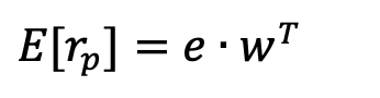
   where e is a (nx1 column vector) matrix of the expected returns for each asset: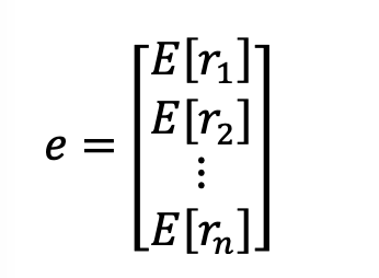

   

   and w is a matrix (nx1 column vector) matrix of the weights of each asset within the portfolio.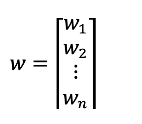

   

   For example:

   >>> weights = [[0.3, 0.4, 0.3]]
   >>> returns = [[0.12, 0.10, 0.05]]
   >>> portfolio_return(weights, returns)
   0.0910
   

2. Write a new implementation of the bond_price(fv, c, n, m, ytm) function to calculate and return the price of a bond using linear algebra. The parameters are:
   fv is the future (maturity) value of the bond;
   c is the annual coupon rate expressed as percentage per year;
   n is the number of years until maturity;
   m is the number of coupon payments per year;
   and ytm, the annualized yield to maturity of the bond
   

   For example:

   >>> bond_price(1000, 0.08, 5, 2, 0.08) # coupon bond at par
   999.9999999999998
   >>> bond_price(1000, 0.08, 5, 2, 0.09) # coupon bond at discount
   960.4364091144498
   >>> bond_price(1000, 0.00, 5, 2, 0.09) # zero-coupon bond
   643.927682030043
   

   Implementation Notes:

   • Your function must use a matrix algebra (no loop with an accumulator pattern or recursion) and requires no if-elif-else logic. The price of the bond is given by the present values of the cashflows of that bond, as represented by this matrix multiplication: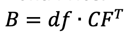

     

     where df is the matrix of discount factors for the bond’s payments, CF is a matrix of the bond’s cashflows, and the result B is a matrix containing the price of the bond.

   • Re-use your bond_cashflows(fv, c, n,m) function from a2task1 to find the cashflows associated with this bond.

   • Re-use your discount_factors(r, n, m) function from a2task1 to calculate the relevant discount factors.

3. Write a new implementation of the bond_duration(fv, c, n, m, ytm) function to calculate and return the annulized duration of a bond using linear algebra. The parameters are:
   fv is the future (maturity) value of the bond;
   c is the annual coupon rate expressed as percentage per year;
   n is the number of years until maturity;
   m is the number of coupon payments per year;
   and ytm, the annualized yield to maturity of the bond
   

   For example:

   >>> bond_duration(1000, 0.05, 2, 2, 0.05) # coupon bond at par
   >>> 1.9280117816050262
   >>> bond_duration(1000, 0.00, 2, 2, 0.05) # zero coupon bond
   >>> 2.0
   >>>
   >>> bond_duration(1000, 0.05, 10, 2, 0.03) # coupon bond at premium
   >>> 8.169425098281545
   

   Implementation Notes:

   • Your function must use a matrix algebra (no loop with an accumulator pattern or recursion) and requires no if-elif-else logic. The duration of the bond is computed using by the cashflows, discount factors, and payment times of that bond, as represented by this matrix multiplication:

     

     where CF is a matrix of the bond’s cashflows; df is a matrix of discount factors for the bond’s payments, T is a matrix of the cashflow times, and B is a matrix containing the price of the bond.

   • Re-use your cashflow_times(n,m) function from a3task1 to find the times of the cashflows of this bond.

   • Re-use your bond_cashflows(fv, c, n, m) function from a3task1 to find the cashflows associated with this bond.

   • Re-use your discount_factors(r, n, m) function from a3task1 to calculate the relevant discount factors.

4. The bootstrap method is a technique to find the implied prices of zero-coupon bonds (i.e., implied discount factors) by using the casflows and prices of some coupon-paying bonds at similar maturities.

   Write the function bootstrap(cashflows, prices) to implement the bootstrap method. This function will take parameters cashflows, which is a matrix (2-dimensional list) containing the cashflows for some bonds, and prices which is a column matrix (2-dimensional list) containing the prices of these bonds.

   We can find the prices of the implied zero-coupon bonds (i.e., discount factors) using this equation:

   

   where P is a matrix containing the price of the bond, CF is the matrix of the bond’s cashflows, and D is the matrix of implied discount factors.

   For example:

   >>> CF = [[105,0,0],[6,106,0],[7,7,107]]
   >>> P = [[99.5], [101.25], [100.35]]
   >>> D = bootstrap(CF, P)
   >>> print_matrix(CF, 'Bond Cashflows')
   Bond Cashflows = 
   [[105.00, 0.00, 0.00]
    [6.00, 106.00, 0.00]
    [7.00, 7.00, 107.00]]
   >>> print_matrix(P, 'Bond Prices')
   Bond Prices = 
   [[99.50]
    [101.25]
    [100.35]]
   >>> print_matrix(D, 'Implied Discount Factors') 
   Implied Discount Factors = 
   [[0.95]
    [0.90]
    [0.82]]
   >>> D
   [[0.9476190476190477], [0.9015498652291104], [0.8168768000940457]]
   

   Notes:

   • Your function must use your matrix algebra functions (no loops).

Submitting Your Work

20 points; will be assignmed by code review

Use the link to GradeScope (left) to submit your work.

Be sure to name your files correctly!

Under the heading for Assignment 4, attach these 4 required files: a2task1.py, a4task1.py, a4task2.py, and a4task3.py.

When you upload the files, the autograder will test your functions/programs.

*   Why does this happen? When the autograder imports your file, the `print` 
    statement(s) execute (at import time), which causes this error.

*   You can prevent this error by not having any `print` statements in the global scope.
    Instead, create an `if __name__ == '__main__':` section at the bottom of the file, and
    put any test cases/print statements in that controlled block. For example:

        if __name__ == '__main__':

            ## put test cases here:
            print('fv_lump_sum(0.05, 2, 100)', fv_lump_sum(0.05, 2, 100))

*   `print` statements inside of functions do not cause this problem.

Notes:

• You may resubmit multiple times, but only the last submission will be graded.