Assignment 6
Discussion on Wednesday 2/25/26
Workshop in class on Monday 3/2/26, Wednedsay 3/4/26
Submission due by 9:00 p.m. on Friday 3/6/26.
Preliminaries
In your work on this assignment, make sure to abide by the collaboration policies of the course.
For each problem in this problem set, we will be writing or evaluating some Python code. You are encouraged to use the Spyder IDE which will be discussed/presented in class, but you are welcome to use another IDE if you choose.
If you have questions while working on this assignment, please post them on Piazza! This is the best way to get a quick response from your classmates and the course staff.
Programming Guidelines
-
Refer to the class Coding Standards for important style guidelines. The grader will be awarding/deducting points for writing code that comforms to these standards.
-
Every program file must begin with a descriptive header comment that includes your name, username/BU email, and a brief description of the work contained in the file.
-
Every function must include a descriptive docstring that explains what the function does and identifies/defines each of the parameters to the function.
-
Your functions must have the exact names specified below, or we won’t be able to test them. Note in particular that the case of the letters matters (all of them should be lowercase), and that some of the names include an underscore character (
_). -
If a function takes more than one input, you must keep the inputs in the order that we have specified.
-
You should not use any Python features that we have not discussed in class or read about in the textbook.
-
Your functions do not need to handle bad inputs – inputs with a type or value that doesn’t correspond to the description of the inputs provided in the problem.
-
You must test each function after you write it.
Warnings: Individual Work, Generative AI, and Academic Conduct!!
-
This is an individual assignment. You may discuss the problem statement/requirements, Python syntax, test cases, and error messages with your classmates. However, each student must write their own code without copying or referring to other student’s work.
-
It is strictly forbidden to use any code that you find from online websites including but not limited to as CourseHero, Chegg, or any other sites that publish homework solutions.
-
It is strictly forbidden to use any generative AI (e.g., ChatGPT, Claude, Gemini, CoPilot or any similar tools**) to write solutions for any assignment.
Students who submit work that is not authentically their own individual work will earn a grade of 0 on this assignment and a reprimand from the office of the Dean.
If you have questions while working on this assignment, please post them on Piazza! This is the best way to get a quick response from your classmates and the course staff.
Objective and Overview
Objective: Learn about the bionomial trees and the binomial option pricing model as a discrete-time approach to simulating stock price movements and valuing European and American style options. In addition, you will gain practice with writing user-defined classes, inheritance, loops, and 2-d lists.
Overview: In this assignment, you will develop some user defined classes and methods to implement binomial trees and to compute option prices using the binomial option pricing model, which provides a good approximation of option prices.
Background: Options are derivative contracts, the eventual value of which depends on some underlying asset (i.e., a stock) at a maturity (expiration) time in the future.
-
Read about options in general on Wikipedia.
-
In this assignment, we will implement the binomial option pricing model. Read about the binomial option pricing model on Wikipedia.
We assume that the price of the underlying asset follows a binomial distribution of possible values. At each period, the underlying asset can either move up or down, according to some risk-neutral probability (explained below). Over subsequence periods, the underlying asset can again move up or down from the previous period.
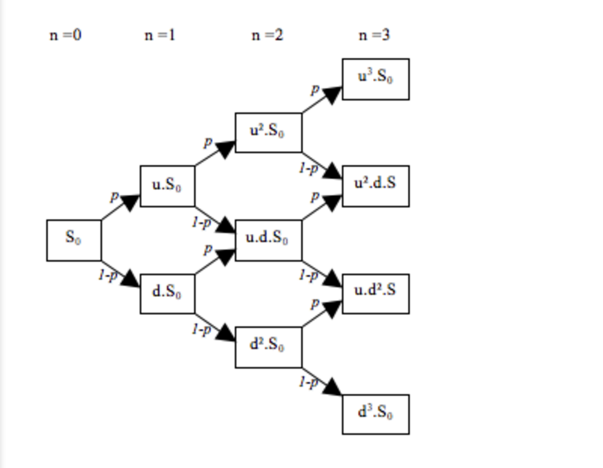
At the limit, the binomial distribution will approximate the normal distribution, so this model gives us a discrete approximation that will give us option prices that are similar to what we would achieve with a continuous-time approach (i.e., Black-Scholes).
Task 1: Creating Binomial Stock Price Trees
30 points; individual-only
Do all of your work for Task 1 of this assignment in a file called a6task1.py.
As with previous assignments, you must use Python lists and loops to develop your solution.
You may not use built-in packages such as numpy or pandas.
To begin, assume that a stock is currently priced at $90, and we want to consider price movements over 6 months (0.5 years), which we further break down into 2 discrete time periods (i.e., of 0.25 years each). Here is a binomial tree illustrating the potential stock price paths over 2 periods, from an initial price of $90:
BinomialTree (s=90, stdev=0.3, rf=0.06, div=0, t=0.5 years, nper=2)
 90.00    106.15    125.19
           78.63     92.74
                     68.70
The binomial price tree will be encapsulated within a class BinomialTree, which will
develop a recombinant binomial tree suitable for any underlying asset, e.g., a stock.
The class will have the following data attributes:
sis the initial underlying (e.g. stock) price nowstdevis the annualized standard deviation of the returns on srfis the annualized risk-free ratedivis the annualized divident yieldtis the time to maturity (in years)nperis number of periods to use in the bionomial tree
In addition, the BinomialTree will calculate and store several additional data
attributes, representing parameters used in the calculation of the binomial price tree.
-
Write the constructor
__init__(self, s, stdev, rf, div, years, nper), which will initialize aBinomialTreeobject.In addition, the constructor of the
BinomialTreewill call a helper method to build the binomial tree as a 2-dimensional list (upper right triangle of a matrix). Seebuild_treebelow.Here is an example of creating a
BinomialTreeobject, and printing it out using the__repr__method (See below):>>> bt = BinomialTree (90, 0.3, 0.06, 0, 0.5, 2) >>> bt # calls the __repr__ method BinomialTree (s=90, stdev=0.3, rf=0.06, div=0, t=0.5 years, nper=2)
-
Write the
__repr__method to obtain a beautifully-formatted string representation of theBinomialTreeobject.To begin, the method should print out the data attributes of the object, i.e.:
>>> bt = BinomialTree (90, 0.3, 0.06, 0, 0.5, 2)
>>> bt
BinomialTree (s=90, stdev=0.3, rf=0.06, div=0, t=0.5 years, nper=2)
-
Write the helper method
build_tree(self), which takes no parameters.This method should build a binomial tree (as a 2-d list), which will simulate the price movements of the s asset. Store the 2-d list as a data attribute of this class called
tree.To begin,
build_treeshould calculate and store the parametersh,uandd, which will be needed to build out the tree.his the length of each time period, which can be computed ash = t/n.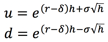
For each period, we assume the stock has a chance of moving up or down, and we calculate the prices in the states up and down using the factors
uandd. The price in the up-state isutimes the previous price, and the price in the down-state usdtimes the previous price.A First Example:
>>> # here we consider a one-period model, which has only two possible stock price outcomes after 1 year:
>>> bt = BinomialTree (90, 0.3, 0.06, 0, 1, 1)
>>> bt.tree # access the 2-d list
[[90, 128.99964731043062], [0.0, 70.79650749598981]]
Notice that
bt.treeis a 2-d list of values. We can visualizebt.treebetter using theprint_matrixfunction that you wrote in Assignment 4, as it helps line up the rows correctly:>>> from a4task1 import print_matrix >>> bt = BinomialTree (90, 0.3, 0.06, 0, 1, 1) >>> print_matrix(bt.tree) [[90, 129] [0.0, 70.80]]
Notice also that this is a 2-d list, with values in the upper-right triangle only. The lower-left triangle should have 0s.
In the next part (number 4, below), you will enhance the
__repr__method to produce a beaut-fully-formatted binomial tree, but for now usingprint_matrixwill suffice.A Second Example:
>>> from a4task1 import print_matrix
>>> # here we consider five possible stock price outcomes over the next 1 year:
>>> bt = BinomialTree (90, 0.3, 0.06, 0, 1, 5)
>>> print_matrix(bt.tree)
[[90.00, 104.16, 120.56, 139.53, 161.49, 186.91]
 [0.00, 79.65, 92.19, 106.69, 123.49, 142.92]
 [0.00, 0.00, 70.49, 81.59, 94.43, 109.29]
 [0.00, 0.00, 0.00, 62.38, 72.20, 83.57]
 [0.00, 0.00, 0.00, 0.00, 55.21, 63.90]
 [0.00, 0.00, 0.00, 0.00, 0.00, 48.86]]
Notice again that this is a 2-d list, with values in the upper-right triangle only. The lower-left triangle should have 0s.
Notes:
-
Re-use your code! Your
build_treemethod should use the binomial parameters that are stored as data attributes of theBinomialTreeobject. -
Call this method as the last line of the constructor, so that upon creating the
BinomialTreeobject the tree is initialized and ready to use. -
The initial underlying price
Swill be the root (left-most) node of the price tree. As such, you will need to create a 2-dimensional list of sizenper+1byn+1(See example above) to be able to createnperdiscrete periods after the initial period.
-
-
Return to your
__repr__method, to create a beautifully-formatted representation of yourBinomialTreeas an upper-right triangle (with bottom-left elements not shown).Example:
>>> # 1 year, 2 periods
>>> bt = BinomialTree (90, 0.3, 0.06, 0, 1, 2)
>>> bt
BinomialTree (s=90, stdev=0.3, rf=0.06, div=0, t=1 years, nper=2)
     90.00    114.66    146.07
               75.01     95.57
                         62.52
Notes:
-
You should always assume that the 2-dimensional list is a square, but that you will only print out the upper-right triangle of the matrix.
-
The printout must have each row on its own line, and use tabs or spaces as needed to create a tree-like illustration.
-
Print each number with 2 digits of precision after the decimal point (but don’t change the underlying data in the 2d list, which must continue to be numeric).
Additional Examples:
>>> # 1 year, 5 periods
>>> bt = BinomialTree (90, 0.3, 0.06, 0, 1, 5)
>>> bt
BinomialTree (s=90, stdev=0.3, rf=0.06, div=0, t=1 years, nper=5)
     90.00    104.16    120.56    139.53    161.49    186.91
               79.65     92.19    106.69    123.49    142.92
                         70.49     81.59     94.43    109.29
                                   62.38     72.20     83.57
                                             55.21     63.90
                                                       48.86

>>> # 1 year, 10 periods
>>> bt = BinomialTree (90, 0.3, 0.06, 0, 1, 10)
>>> bt
BinomialTree (s=90, stdev=0.3, rf=0.06, div=0, t=1 years, nper=10)
     90.00     99.55    110.12    121.80    134.73    149.03    164.85    182.34    201.69    223.10    246.78
               82.35     91.09    100.75    111.45    123.27    136.36    150.83    166.84    184.54    204.13
                         75.34     83.34     92.19    101.97    112.79    124.76    138.00    152.65    168.85
                                   68.94     76.25     84.35     93.30    103.20    114.15    126.27    139.67
                                             63.08     69.77     77.17     85.37     94.43    104.45    115.53
                                                       57.71     63.84     70.61     78.11     86.40     95.57
                                                                 52.80     58.41     64.61     71.46     79.05
                                                                           48.31     53.44     59.11     65.39
                                                                                     44.21     48.90     54.09
                                                                                               40.45     44.74
                                                                                                         37.01
-
-
Create mutator methods (e.g.,
set_s) to be able to change each of the data attributes of the object. Changing any data attribute will change the prices in the tree, so it is important that these methods also call thebuild_treemethod.Here are some examples:
>>> bt = BinomialTree (90, 0.3, 0.06, 0, 1, 4)
>>> bt
BinomialTree (s=90, stdev=0.3, rf=0.06, div=0, t=1 years, nper=4)
     90.00    106.15    125.19    147.64    174.13
               78.63     92.74    109.38    129.00
                         68.70     81.03     95.57
                                   60.03     70.80
                                             52.45
Changing the
sresults in shifting the starting node, and also the proportional movements from this starting point:>>> bt.set_s(100) >>> bt BinomialTree (s=100, stdev=0.3, rf=0.06, div=0, t=1 years, nper=4) 100.00 117.94 139.10 164.05 193.48 87.37 103.05 121.53 143.33 76.34 90.03 106.18 66.70 78.66 58.27Increasing the standard deviation results in widening the distribution of prices (both upper and lower) branches:
>>> bt.set_stdev(0.4)
>>> bt
BinomialTree (s=100, stdev=0.4, rf=0.06, div=0, t=1 years, nper=4)
    100.00    123.99    153.73    190.60    236.32
               83.11    103.05    127.76    158.41
                         69.07     85.64    106.18
                                   57.41     71.18
                                             47.71
Increasing the number of periods results in both more nodes, and also smaller price movements in each node:
>>> bt.set_nper(5)
>>> bt
BinomialTree (s=100, stdev=0.4, rf=0.06, div=0, t=1 years, nper=5)
    100.00    121.03    146.49    177.30    214.59    259.72
               84.63    102.43    123.97    150.05    181.60
                         71.62     86.69    104.92    126.98
                                   60.61     73.36     88.79
                                             51.30     62.09
                                                       43.41
Decreasing the risk-free rate decreases the amount of the up and down movements between each node:
>>> bt.set_rf(0.03)
>>> bt
BinomialTree (s=100, stdev=0.4, rf=0.03, div=0, t=1 years, nper=5)
100.00    120.31    144.74    174.13    209.50    252.04
           84.12    101.21    121.76    146.49    176.24
                     70.77     85.14    102.43    123.23
                               59.53     71.62     86.17
                                         50.08     60.25
                                                   42.13
Task 2: Binomial Options Pricing
50 points; individual-only
Overview and Methodology
The value of an option depends on the price of the underlying security (e.g., stock). The bionomial option pricing model uses the value of an option at maturity (given the price of the underlying), and then works backwards to find the value of the option today.
Consider this one-period example for a European call option, which gives the right (but not the obligation) to purchase a stock in one year:
>>> # consider the posisble stock price in one year:
>>> bt = BinomialTree(25, 0.25, 0.05, 0.03, 1, 1)
>>> print(bt)
BinomialTree (s=25, stdev=0.25, rf=0.05, div=0.03, t=1 years, nper=1)
     25.00     32.75
               19.86
>>> # the payoff of the option at maturity (time 1) depends on the
    # underlying price and the strike price:
>>> call = BinomialEuroCallOption(25, 22, 0.25, 0.05, 0.03, 1, 1)
European Call Option Tree (s=25, x=22, stdev=0.25, rf=0.05, div=0.03, t=1 years, nper=1)
      4.48     10.75
                0.00
The call option’s value depends on the stock price at maturity and the execute price. In the above example, we assume that after 1 year, the stock price can rise to $32.75 or fall to $19.86.
The value of the call option is C = MAX(S - X, 0).
The payoff value of the stock option in the “up” state is $32.75 - $22 = $10.75. The payoff value of the option in the “down” state would be $19.86 - $22 = $-2.14 ... therefore the option holder will not execute the option, so it’s value is $0.
Given these two possible states, we find the value of the option at time 0 (today) by finding the “expected value” at maturity (using the risk-neutral probability of the “up” and “down” states), and discount this expected value to the present.
The same procedure will work for any number of binomial periods.
Call option value
At maturity (in the right-most column), the value of a call option at maturity is simply
its payoff, i.e., the amount by which the stock price in the corresponding node exceeds
the strike price: C = MAX(S - X, 0).
Once the right-most nodes have been calculated, we can work backwords for all other nodes. In general, the value of the call option in a given node is calculated by:

where Ci,j is the option’s value for node in position i,j of the tree,
and depends on the value in the nodes Ci, j+1 and Ci+1, j+1.
Continue to work right-to-left until you reach the root of the tree.
Put option value
At maturity (in the right-most column), the value of a put option at maturity is simply
its payoff, i.e., the amount by which the strike price in the corresponding node exceeds
the stock price: P = MAX(X - S, 0).
Once the right-most nodes have been calculated, we can work backwords for all other nodes. In general, the value of the put option in a given node is calculated by:

where Pi,j is the option’s value for node in position i,j of the tree,
and depends on the value in the nodes Pi, j+1 and Pi+1, j+1.
Continue to work right-to-left until you reach the root of the tree.
Do the work for this part in a file called a6task2.py. At the top of your file,
you will need to import your work from Task 1, i.e.,
from a6task1 import *
-
Write the class definition for the
BinomialOptionclass, which is a subclass of theBinomialTreefrom Task 1. This object will be an abstract class, i.e., we wil not actually create objects of this type. Rather, we will use it as a building block for several specific sub-classes, which will share most details but implement specific pricing algorithms.The constructor (
__init__method) must take parameters for:s, the price of the underlying (e.g. stock) nowx, the strike price of the optionstdev, the annualized standard deviation of the returns on srf, the annualized risk-free ratediv, the annualized divident yieldt, the time to maturity (in years)nper, number of periods to use in the bionomial tree
The constructor (
__init__method) must begin by calling the superclass constructor, i.e., to initialize the part of theBinomialOptionwhich is aBinomialTreeobject. To do so, use the syntax:super().__init__( < parameters> )
to supply the constructor parameters required for class
BinomialTree.Next, the constructor must store the data attribute
x, which is specific to theBinomialOptionclass (i.e., not part of the superclass).Finally, the constructor will call a helper method
build_option_tree. This method will be implemented on each of various subclasses, corresponding to specific type of options. It is not possible to call this method on the genericBinomialOption, but polymorphism will handle the detail of calling the correct subclass version of the method. Add the method call to the constructor now, but you will test it when you create objects of the subclass (See below). -
Write the class definition for the
BinomialEuroCallOptionclass, which is a subclass of theBinomialOptionsuperclass.The
BinomialEuroCallOptionwill provide a concrete implementation of the option pricing algorithm for a European-style call option, which is exercisable only at maturity.You do not need to write a constructor for this class! The constructor for the superclass
BinomialOptiondoes exactly what we need.Write a
__repr__method to produce a string representation of this object. To begin, you may print out the data attributes:>>> call = BinomialEuroCallOption(25, 22, 0.25, 0.05, 0.03, 1, 1) >>> call European Call Option Tree (s=25, x=22, stdev=0.25, rf=0.05, div=0.03, t=1 years, nper=1)
Next, write the method
build_option_treemethod, which will calculate the option value at each node in the tree, and save it as a data attribute calledoption_tree.-
Create an empty 2-dimensional list of the appropriate dimensions to hold the option values for each node in the tree.
-
Use the superclass’s binomial tree, e.g.,
self.tree, to find the value of the underlying in each node. Begin with the right-most column, and compute the value of the European Call Option in each node, i.e.,MAX(S - X, 0). -
Work right-to-left to find the option value in each preceding node. The value in each preceding node is the weighted-average of the up and down states reachable from that node.
Update your
__repr__method to display theoption_treewith formatting, e.g.,>>> call = BinomialEuroCallOption(25, 22, 0.25, 0.05, 0.03, 1, 1) >>> call European Call Option Tree (s=25, x=22, stdev=0.25, rf=0.05, div=0.03, t=1 years, nper=1) 4.48 10.75 0.00Here is another example with which to test your work – an “in-the-money” call option on a dividen-paying stock, with 1 years to maturity and 2 periods in the binomial option pricing process.
>>> call = BinomialEuroCallOption(25, 22, 0.25, 0.05, 0.03, 1, 2)
>>> call
European Call Option Tree (s=25, x=22, stdev=0.25, rf=0.05, div=0.03, t=1 years, nper=2)
      4.49      8.23     14.32
                1.56      3.51
                          0.00
Here is a second example, a call option on a dividen-paying stock, with 0.25 years to maturity, calculated with 5 periods in the bionomial process.
>>> call = BinomialEuroCallOption(25, 22, 0.25, 0.05, 0.03, 0.25, 5)
>>> call
European Call Option Tree (s=25, x=22, stdev=0.25, rf=0.05, div=0.03, t=0.25 years, nper=5)
      3.32      4.58      6.05      7.67      9.40     11.23
                2.15      3.20      4.55      6.08      7.71
                          1.16      1.95      3.12      4.57
                                    0.41      0.85      1.76
                                              0.00      0.00
                                                        0.00
Here is another example: For example, here is the European call option value tree for these parameters:
>>> # s = 90, x = 100, sigma = 0.3, rf = 0.06, div = 0.02, t = 0.25, n = 10:
>>> call = BinomialEuroCallOption(90, 100, 0.3, 0.06, 0.02, 0.25, 10)
>>> call
European Call Option Tree (s=90, x=100, stdev=0.3, rf=0.06, div=0.02, t=0.25 years, nper=10)
  2.11      3.32      5.10      7.63     11.06     15.45     20.71     26.58     32.76     39.25     46.08
            0.96      1.63      2.71      4.39      6.90     10.47     15.17     20.77     26.66     32.86
                      0.33      0.61      1.11      2.00      3.52      6.02      9.88     15.21     20.83
                                0.06      0.13      0.27      0.56      1.15      2.35      4.82      9.90
                                          0.00      0.00      0.00      0.00      0.00      0.00      0.00
                                                    0.00      0.00      0.00      0.00      0.00      0.00
                                                              0.00      0.00      0.00      0.00      0.00
                                                                        0.00      0.00      0.00      0.00
                                                                                  0.00      0.00      0.00
                                                                                            0.00      0.00
                                                                                                      0.00
-
-
Revisit the
BinomialOptionto add mutator methods for all data attributes. Follow the naming conventionset_<attribute_name>, e.g.,set_x. These methods must call the superclass version of the mutator method (So that the superclass will rebuild its price tree), and then must recalculate the option’s value by calling thebuild_option_treemethod again.Here are several examples of using the mutator methods (by calling them on the subclass).
>>> call = BinomialEuroCallOption(25, 22, 0.25, 0.05, 0.03, 0.25, 5)
>>> call
European Call Option Tree (s=25, x=22, stdev=0.25, rf=0.05, div=0.03, t=0.25 years, nper=5)
      3.32      4.58      6.05      7.67      9.40     11.23
                2.15      3.20      4.55      6.08      7.71
                          1.16      1.95      3.12      4.57
                                    0.41      0.85      1.76
                                              0.00      0.00
                                                        0.00

>>> call.set_x(20) # lower the strike price; call becomes more valuable
>>> call
European Call Option Tree (s=25, x=20, stdev=0.25, rf=0.05, div=0.03, t=0.25 years, nper=5)
      5.10      6.50      8.04      9.66     11.39     13.23
                3.79      5.09      6.54      8.08      9.71
                          2.58      3.74      5.11      6.57
                                    1.50      2.46      3.76
                                              0.60      1.25
                                                        0.00

>>> call.set_years(1) # lengthen the maturity to 1 year; call becomes more valuable
>>> call
European Call Option Tree (s=25, x=20, stdev=0.25, rf=0.05, div=0.03, t=1 years, nper=5)
      5.76      8.32     11.54     15.36     19.69     24.61
                3.57      5.59      8.35     11.78     15.67
                          1.83      3.23      5.45      8.52
                                    0.61      1.31      2.81
                                              0.00      0.00
                                                        0.00

>>> call.set_rf(0.10) # set risk free rate higher; call becomes more valuable
>>> call
European Call Option Tree (s=25, x=20, stdev=0.25, rf=0.1, div=0.03, t=1 years, nper=5)
      6.47      9.28     12.74     16.81     21.50     26.89
                4.22      6.53      9.59     13.26     17.50
                          2.31      4.04      6.68      9.98
                                    0.85      1.84      3.98
                                              0.00      0.00
                                                        0.00

>>> call.set_stdev(0.4) # increase standard deviation; call becomes more valuable
>>> call
European Call Option Tree (s=25, x=20, stdev=0.4, rf=0.1, div=0.03, t=1 years, nper=5)
      7.34     11.49     17.28     24.84     34.15     45.58
                4.14      7.07     11.59     17.98     25.86
                          1.85      3.56      6.68     12.06
                                    0.48      1.08      2.42
                                              0.00      0.00
                                                        0.00
Add a
valuemethod, that will return the value of the option at time 0.>>> call = BinomialEuroCallOption(25, 22, 0.25, 0.05, 0.03, 0.25, 5) >>> call.value() # returns the value as a floating-point number 3.3190742916994407
-
Write the class definition for the
BinomialEuroPutOptionclass, which is a subclass of theBinomialOptionsuperclass.The
BinomialEuroPutOptionwill provide a concrete implementation of the option pricing algorithm for a European-style put option, which is exercisable only at maturity.You do not need to write a constructor for this class! The constructor for the superclass
BinomialOptiondoes exactly what we need.Write a
__repr__method to produce a string representation of this object. To begin, you may print out the data attributes:>>> put = BinomialEuroPutOption(25, 22, 0.25, 0.05, 0.03, 1, 1) >>> put European Put Option Tree (s=25, x=22, stdev=0.25, rf=0.05, div=0.03, t=1 years, nper=1)
Next, write the method
build_option_treemethod, which will calculate the option value at each node in the tree, and save it as a data attribute calledoption_tree.-
Create an empty 2-dimensional list of the appropriate dimensions to hold the option values for each node in the tree.
-
Use the superclass’s binomial tree, e.g.,
self.tree, to find the value of the underlying in each node. Begin with the right-most column, and compute the value of the European Put Option in each node, i.e.,MAX(X - S, 0). -
Work right-to-left to find the option value in each preceding node. The value in each preceding node is the weighted-average of the up and down states reachable from that node.
Update your
__repr__method to display theoption_treewith formatting, e.g.,>>> put = BinomialEuroPutOption(25, 22, 0.25, 0.05, 0.03, 1, 1) >>> put European Put Option Tree (s=25, x=22, stdev=0.25, rf=0.05, div=0.03, t=1 years, nper=1) 1.14 0.00 2.14
-
The main difference between American options and European options is that European options are only exercisable at maturity. By contrast, American options are exercisable any time before maturity. That is, the holder of the option may choose to exercise at any time, if this is worth more than holding the option.
For American call options, early exercise is never worthwhile. Rather, the live value of the option is worth more than the early-exercise value. If the owner of the American call option wants out, they are best off simply selling the option. Therefore the value of the American call option is the same as the European call option.
Exercising an American put option might* be worth more than the live value of holding the option to maturity (i.e., European put options, depending on the level of interest rates and dividends). In this case, we need to check at each node whether early-exercise is optimal.
As such, the payoff at each node in the binomial option value tree is given by the maximum of the live-value of the option or the immediate exercise and option payoff:

where Pi,j is the option’s value for node in position i,j of the tree,
and depends on the value in the nodes Pi, j+1 and Pi+1, j+1,
and Si,j is the value of the underlyingtock in position i,j of the tree.
-
Write the class definition for the
BinomialAmericanPutOptionclass, which is a subclass of theBinomialOptionsuperclass.The
BinomialAmericanPutOptionwill provide a concrete implementation of the option pricing algorithm for an American-style put option, which is exercisable at any time until maturity.You do not need to write a constructor for this class! The constructor for the superclass
BinomialOptiondoes exactly what we need.Write a
__repr__method to produce a string representation of this object. To begin, you may print out the data attributes:>>> put = BinomialAmericanPutOption(25, 22, 0.25, 0.05, 0.03, 1, 1) >>> put American Put Option Tree (s=25, x=22, stdev=0.25, rf=0.05, div=0.03, t=1 years, nper=1)
Next, write the method
build_option_treemethod, which will calculate the option value at each node in the tree, and save it as a data attribute calledoption_tree.-
Create an empty 2-dimensional list of the appropriate dimensions to hold the option values for each node in the tree.
-
Use the superclass’s binomial tree, e.g.,
self.tree, to find the value of the underlying in each node. Begin with the right-most column, and compute the value of the European Call Option in each node, i.e.,MAX(X - S, 0). -
Work right-to-left to find the option value in each preceding node. The value in each preceding node is the maximum of:
1 - the “live value” of the option, i.e., weighted-average of the up and down states reachable from that node, discounted to present value.
2 - the “exercise value” of the option, i.e., the value obtains from immediate exercise in this node:
MAX(X - S, 0).Update your
__repr__method to display theoption_treewith formatting, e.g.,>>> put = BinomialAmericanPutOption(25, 22, 0.25, 0.05, 0.03, 1, 1) >>> put American Put Option Tree (s=25, x=22, stdev=0.25, rf=0.05, div=0.03, t=1 years, nper=1) 1.14 0.00 2.14
What’s the difference? Consider these two otherwise identical options:
>>> put = BinomialEuroPutOption(25, 25, 0.25, 0.06, 0.02, 1, 4)
>>> put
European Put Option Tree (s=25, x=25, stdev=0.25, rf=0.06, div=0.02, t=1 years, nper=4)
      1.94      0.68      0.00      0.00      0.00
                3.12      1.30      0.00      0.00
                          4.81      2.48      0.00
                                    7.01      4.74
                                              9.22
>>> put = BinomialAmericanPutOption(25, 25, 0.25, 0.06, 0.02, 1, 4)
>>> put
American Put Option Tree (s=25, x=25, stdev=0.25, rf=0.06, div=0.02, t=1 years, nper=4)
      2.03      0.68      0.00      0.00      0.00
                3.29      1.30      0.00      0.00
                          5.14      2.48      0.00
                                    7.29      4.74
                                              9.22
The American put option is worth a bit more than they European option, because of the possibility of early exercise.
-
Submitting Your Work
10 points; will be assignmed by code review
Use the link to GradeScope (left) to submit your work.
Be sure to name your files correctly!
Under the heading for Assignment 7, attach these 2 required files:
a6task1.py and a6task2.py.
When you upload the files, the autograder will test your functions/programs.
Warning: Beware of Global print statements
- The autograder script cannot handle
printstatements in the global scope, and their inclusion causes this error:

*   Why does this happen? When the autograder imports your file, the `print`
    statement(S) execute (at import time), which causes this error.

*   You can prevent this error by not having any `print` statements in the global scope.
    Instead, create an `if __name__ == '__main__':` section at the bottom of the file, and
    put any test cases/print statements in that controlled block. For example:

        if __name__ == '__main__':

            ## put test cases here:
            print('fv_lump_sum(0.05, 2, 100)', fv_lump_sum(0.05, 2, 100))

*   `print` statements inside of functions do not cause this problem.
Notes:
- You may resubmit multiple times, but only the last submission will be graded.