Assignment 7

Introduction online only 3/17/25
Workshop in class on Wednesday 3/19/25
Submission due by 9:00 p.m. on Friday 3/21/25.

Preliminaries

In your work on this assignment, make sure to abide by the collaboration policies of the course.

For each problem in this problem set, we will be writing or evaluating some Python code. You are encouraged to use the Spyder IDE which will be discussed/presented in class, but you are welcome to use another IDE if you choose.

If you have questions while working on this assignment, please post them on Piazza! This is the best way to get a quick response from your classmates and the course staff.

If you have questions while working on this assignment, please post them on Piazza! This is the best way to get a quick response from your classmates and the course staff.

Objective and Overview

Objective: Develop an intuitive understanding of the Black-Scholes-Merton option pricing formula. Use object-oriented programming, class definintions, inheritance, and polymorphism to create a hierarchy of option classes, and to solve for the implied volatility observed in option prices.

Overview: In this assignment, you will implement some user-defined classes to assist with option pricing using the Black-Scholes formula.

To do so, you will implement a base class to encapsulate the fundamental data members and common calculations used by both call and put options, and then create subclasses to implement call- or put-specific features.

Task 1: Option Pricing using the Black-Scholes-Merton formula

50 points; individual-only

The Black-Scholes model is a mathematical model used for valuing European call and put options.

In this task, you will write several class definitions as well as some client code to implement and test the Black-Scholes pricing formula. Do this entire task in a file called a7task1.py.

1. Write a definition for the base class BSMOption, which encapsulates the data required to do Black-Scholes option pricing formula. The data required include:
   s (the current stock price in dollars),
   x (the option strike price),
   t (the option maturity time in years),
   sigma (the annualized standard deviation of returns),
   rf (the annualized risk free rate of return),
   div (the annualized dividend rate; assume continuous dividends rate),
   

   Create the __init__ and __repr__ methods for the class BSMOption, such that you can create and print out an object like this:

   Example:

   >>> option = BSMOption(100, 100, 0.25, 0.3, 0.06, 0.00)
   >>> print(option)
   s = $100.00, x = $100.00, t = 0.25 (years), sigma = 0.300, rf = 0.060, div = 0.00
   

   Note:

   * The `BSMOption` is a base class (a building block for option classes), but not a 
     concrete option. We cannot compute it's price or delta. Rather, we will create 
     subclasses later to compute the price.
   

   Write a method set_sigma(s), which will make it possible to change the value of the standard deviation (sigma) after object creation. Here is an example of using this method:

   >>> option = BSMOption(100, 100, 0.25, 0.3, 0.06, 0.00)
   >>> print(option)
   s = $100.00, x = $100.00, t = 0.25 (years), sigma = 0.300, rf = 0.060, div = 0.00
   >>> option.set_sigma(0.5)
   >>> print(option)
   s = $100.00, x = $100.00, t = 0.25 (years), sigma = 0.500, rf = 0.060, div = 0.00
   

2. The Black-Scholes-Merton formula for call and put options require the following factors:

   

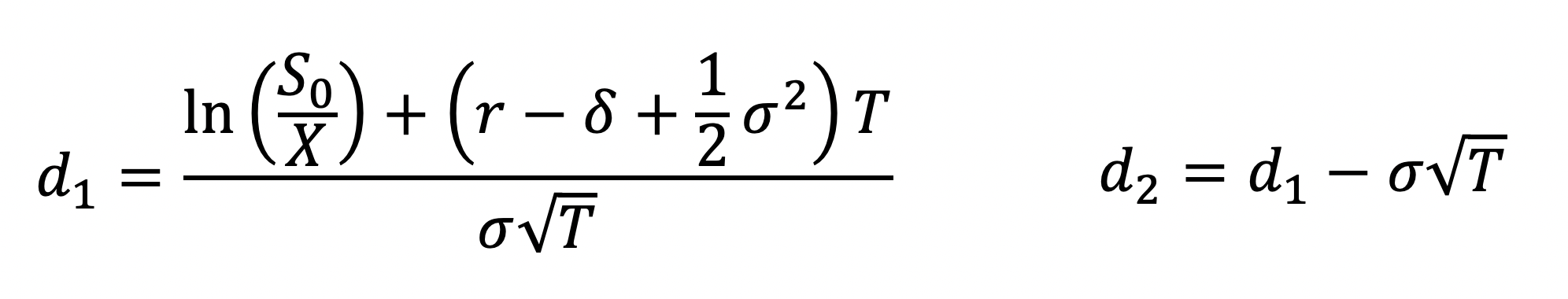
   Create the following 4 methods on the class BSMOption to calculate d1, d2, nd1, and nd2. You should be able to test these formulas as such:

   >>> option = BSMOption(100, 100, 0.25, 0.3, 0.06, 0.00)
   >>> print(option)
   s = $100.00, x = $100.00, t = 0.25 (years), sigma = 0.300, rf = 0.060, div = 0.00
   >>> option.d1()
   0.175
   >>> option.d2()
   0.024999999999999994
   >>> option.nd1()
   0.56946018320767366
   >>> option.nd2()
   0.50997251819523803
   

   Notes:

   • The methods nd1() and nd2() correspond to the expressions N(d1) and N(d2), which are the normal cumulative probability density of d1 and d2 respectively. To calculate this, begin by importing the norm module from the scipy.stats package:

     from scipy.stats import norm
     

   • After importing, you can use the function norm.cdf(x) to find the cumulative probability density of x.

3. Write method declarations on class BSMOption for the methods value(self) and delta(self). These are methods that will be concretely implemented in the subclasses, but we want to have them as part of the interface of the base class. This will be further explained in parts 2 and 3 below. For now, the implementation should merely. print out a brief message and return 0, i.e.,

   >>> option = BSMOption(100, 100, 0.25, 0.3, 0.06, 0.00)
   >>> print(option)
   s = $100.00, x = $100.00, t = 0.25 (years), sigma = 0.300, rf = 0.060, div = 0.00
   >>> option.value()
   Cannot calculate value for base class BSMOption. # print statement
   0 # return value
   >>> option.delta()
   Cannot calculate delta for base class BSMOption. # print statement
   0 # return value
   

4. Write a definition for the class BSMEuroCallOption, which inherits from the base class BSMOption and implements the pricing algorithm for a European-style call option. This new class will have a constructor that takes all of the same parameters, as BSMOption, in the same order, and initializes the base-class object appropriately.

   Your class BSMEuroCallOption must override the __repr__(self) and value(self) methods, to provide a specific implementation appropriate for a European Call option. For example:

   >>> call = BSMEuroCallOption(100, 100, 1, 0.30, 0.06, 0.00)
   >>> print(call)
   BSMEuroCallOption, value = $14.72,
   parameters = (s = $100.00, x = $100.00, t = 1.00 (years), sigma = 0.300, rf = 0.060, div = 0.00) ,
   >>> call.value()
   14.717072420289298
   

   Note that the call option’s __repr__ method calls the option’s value, and uses this value as part of it’s result.

   I recommend that you implement the value method first, and then complete the __repr__ method.

   The European call option’s value is given by this equation:

   

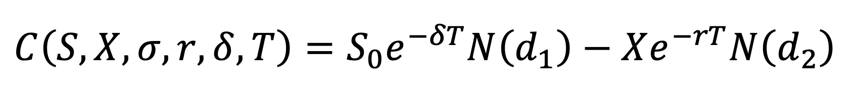
   Note that value method takes no parameters, other than the required reference self. In your implementation, you will use the data members of the base-class BSMOption, as well as the base-class methods nd1() and nd2(). This method will not print anything, but will return the call option’s value.

   Here are some additional examples/test cases:

   >>> # in-the-money (S > X) call option:
   >>> call = BSMEuroCallOption(100, 90, 1.0, 0.30, 0.06, 0.00)
   >>> call.value()
   20.250875968027721
   >>> # out-of-the-money (X > S) call option:
   >>> call = BSMEuroCallOption(90, 100, 1.0, 0.30, 0.06, 0.00)
   >>> call.value()
   9.0162606515961699
   >>> # call on dividend-paying stock:
   >>> call = BSMEuroCallOption(90, 100, 1.0, 0.30, 0.06, 0.04)
   >>> call.value()
   7.3465659048018956
   >>> # call with short maturity:
   >>> call = BSMEuroCallOption(90, 100, 0.25, 0.30, 0.06, 0.04)
   >>> call.value()
   2.1119301352579818
   >>> # call with higher standard deviation:
   >>> call = BSMEuroCallOption(90, 100, 0.25, 0.50, 0.06, 0.04)
   >>> call.value()
   5.3656759063754969
   

5. Write a definition for the class BSMEuroPutOption, which inherits from the base class BSMOption and implements the pricing algorithm for a European-style put option. This new class will have a constructor that takes all of the same parameters, as BSMOption, in the same order, and initializes the base-class object appropriately.

   Your class BSMEuroPutOption must override the __repr__(self) and value(self) methods, to provide a specific implementation appropriate for a European Put option. For example:

   >>> put = BSMEuroPutOption(100, 100, 1, 0.30, 0.06, 0.00)
   >>> print(put)
   BSMEuroPutOption, value = $8.89,
   parameters = (s = $100.00, x = $100.00, t = 1.00 (years), sigma = 0.300, rf = 0.060, div = 0.00) 
   >>> put.value()
   8.8935257787141637
   

   Note that the put option’s __repr__ method calls the option’s value, and uses this value as part of it’s result.

   I recommend that you implement the value method first, and then complete the __repr__ method.

   The European put option’s value is given by this equation:

   

   Note the value method takes no parameters, other than the required reference self. In your implementation, you will use the data members of the base-class BSMOption, as well as the base-class methods nd1() and nd2().

   This method will not print anything, but will return the put option’s value.

   Notes:

   • The value N(-d1) is an area under the normal curve, corresponding to the cumulative probability of a value less than or equal to -d1 standard deviations. This is the same value as the area above d1, i.e., N(-d1) == 1 - N(d1).

   Here are some additional examples/test cases:

   >>> # out-of-the-money (S > X) put option:
   >>> put = BSMEuroPutOption(100, 90, 1.0, 0.30, 0.06, 0.00)
   >>> put.value()
   5.0096839906100996
   >>> # in-the-money (S < X) put option:
   >>> put = BSMEuroPutOption(90, 100, 1.0, 0.30, 0.06, 0.00)
   >>> put.value()
   13.192714010021035
   >>> # put option on dividend-paying stock
   >>> put = BSMEuroPutOption(90, 100, 1.0, 0.30, 0.06, 0.04)
   >>> put.value()
   15.051969739517673
   >>> # put option with short maturity
   >>> put = BSMEuroPutOption(90, 100, 0.25, 0.30, 0.06, 0.04)
   >>> put.value()
   11.518639058139101
   >>> # put option with higher standard deviation
   >>> put = BSMEuroPutOption(90, 100, 0.25, 0.50, 0.06, 0.04)
   >>> put.value()
   14.772384829256616
   

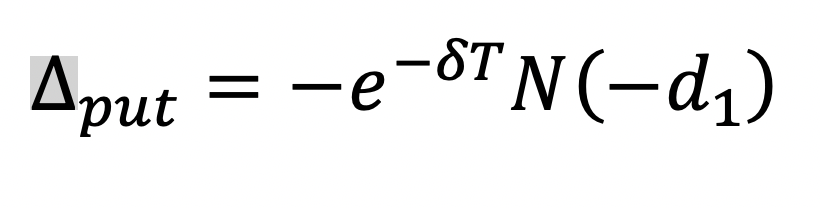
6. Add method declarations on the BSMEuroCallOption and BSMEuroPutOption classes to override the base-class implementation of the delta(self) method. The delta of an option is helpful to create a hedging portfolio to offset the option’s price risk. We can think of an option’s delta as an approximation of the change in the value of this option for a $1 change in price in the underlying stock (i.e., the first derivative of the change in option value with respect to the change in the underlying).

   The detlas for European call and put options are given by these equations:

   
   
   

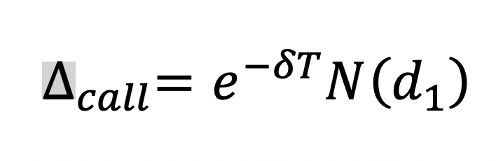
   Note that this method takes no parameters, other than the required reference self. In your implementation, you will use the data members of the base-class BSMOption, as well as the base-class method nd1(). This method will not print anything, but will return the option’s delta value.

   Here are some examples generated using the delta methods on these objects:

   >>> call = BSMEuroCallOption(100, 100, 0.5, 0.25, 0.04, 0.02)
   >>> call.delta()
   0.5520790587734332 
   >>> put = BSMEuroPutOption(100, 100, 0.5, 0.25, 0.04, 0.02)
   >>> put.delta()
   -0.4379707749757349
   >>> # change standard deviation:
   >>> cal.set_sigma(0.5)
   >>> call.delta()
   0.5754543414530255
   >>> put.set_sigma(0.5)
   >>> put.delta()
   -0.4145954922961426
   

Task 2: Client applications using Black-Scholes

30 points; individual-only

Do the work for this part in a file called a7task2.py. At the top of your file, you will need to import your work from Task 1, i.e.,

    from a7task1 import *

1. The option prices shown on a website like Yahoo Finance often show the option prices for otherwise similar options with a wide range of strike prices.

   Write a client-code function generate_option_value_table(s, x, t, sigma, rf, div) (not a class method) which will generate a printout to illustrate the change in option prices with respect to the change in the underlying stock price. The function will require the following parameters:
   s (the current stock price in dollars),
   x (the option strike price),
   t (the option maturity time in years),
   sigma (the annualized standard deviation of returns),
   rf (the annualized risk free rate of return),
   div (the annualized dividend rate; assume continuous dividends rate),
   

   Here is a sample output from this function:

   BSMEuroCallOption, value = $7.44,
   parameters = (s = $100.00, x = $100.00, t = 0.50 (years), sigma = 0.250, rf = 0.040, div = 0.02) 
   BSMEuroPutOption, value = $6.46,
   parameters = (s = $100.00, x = $100.00, t = 0.50 (years), sigma = 0.250, rf = 0.040, div = 0.02)
   
   Change in option values w.r.t. change in stock price:
      price        call value      put value       call delta      put delta
   $   90.00         3.0650         11.9804          0.3227         -0.6673
   $   91.00         3.3990         11.3243          0.3453         -0.6447
   $   92.00         3.7557         10.6910          0.3682         -0.6218
   $   93.00         4.1355         10.0808          0.3914         -0.5987
   $   94.00         4.5385          9.4937          0.4146         -0.5755
   $   95.00         4.9647          8.9299          0.4379         -0.5522
   $   96.00         5.4142          8.3893          0.4611         -0.5289
   $   97.00         5.8869          7.8719          0.4842         -0.5058
   $   98.00         6.3826          7.3776          0.5071         -0.4829
   $   99.00         6.9011          6.9060          0.5298         -0.4603
   $  100.00         7.4421          6.4569          0.5521         -0.4380
   $  101.00         8.0051          6.0300          0.5740         -0.4161
   $  102.00         8.5899          5.6246          0.5954         -0.3946
   $  103.00         9.1958          5.2405          0.6163         -0.3737
   $  104.00         9.8224          4.8771          0.6367         -0.3533
   $  105.00        10.4690          4.5337          0.6565         -0.3335
   $  106.00        11.1352          4.2098          0.6757         -0.3144
   $  107.00        11.8201          3.9047          0.6942         -0.2959
   $  108.00        12.5233          3.6178          0.7120         -0.2781
   $  109.00        13.2439          3.3483          0.7291         -0.2609
   $  110.00        13.9813          3.0957          0.7456         -0.2445
   

   Implementation Notes:

   • This function should create exactly 2 option objects, a call and a put.

   • Inside the function, use a loop to iterate over a range of possible prices. At each price, change the object’s stock price (call.s or put.s), and then use the methods to obtain the options’s value and delta.

2. One limitation of the Black-Scholes model is that while we can observe the current stock price, we cannot know with certainty the appropriate standard deviation to use. However, this limitation can become an advantage, as we can observe stock and option prices in the market, and use the Black-Scholes model to find the implied volatility, i.e., the amount of standard deviation that explains the current option price. The implied volatility tells us how risky the stock is, according to the opinion of options market-makers.

   For example, here is a listing of ~3-month (100 day) call options on Starbucks as of 3/2/2022:

   

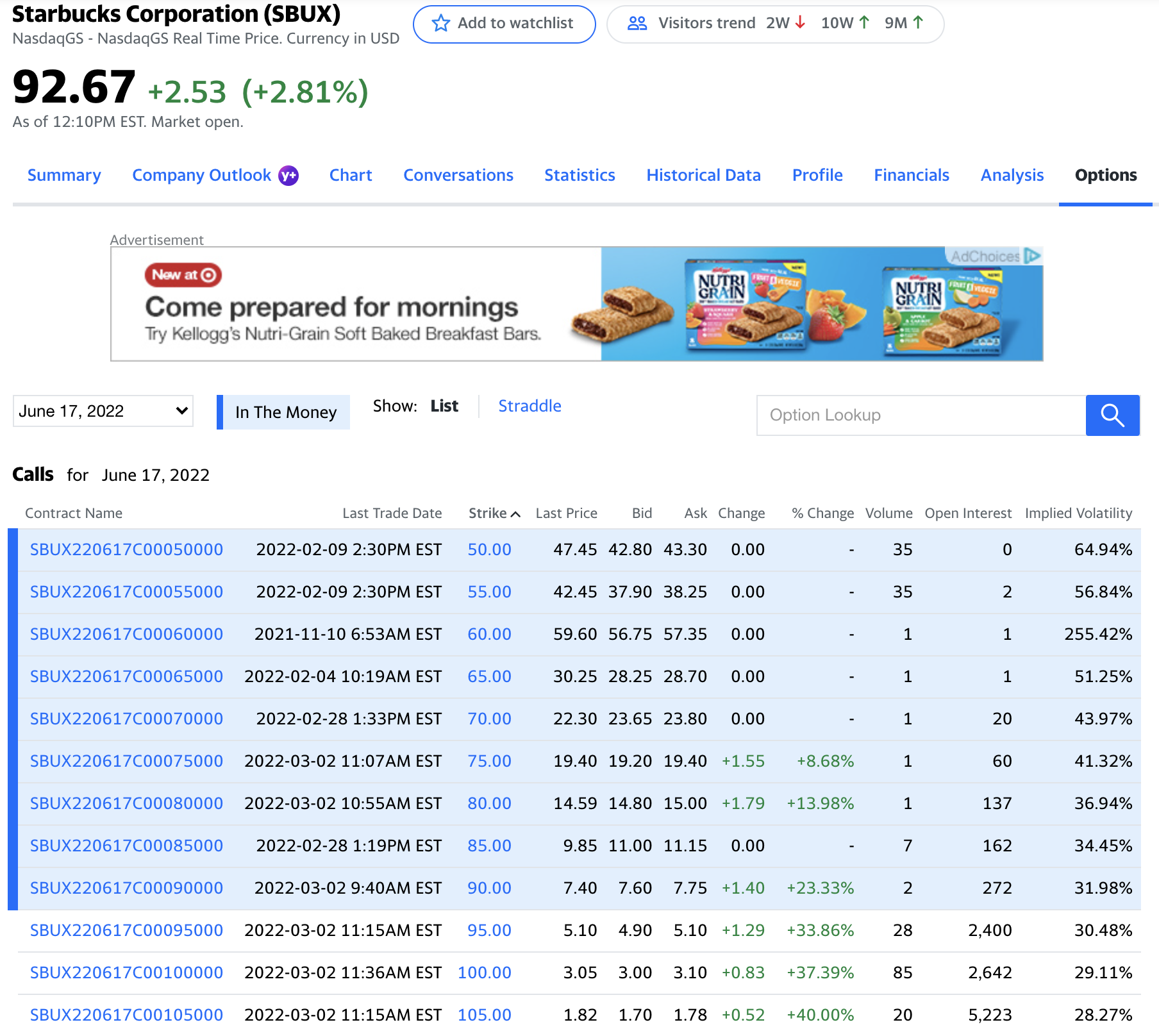
   (source: Yahoo Finance, http://finance.yahoo.com/quote/SBUX/options?p=SBUX)

   Write a client function calculate_implied_volatility(option, value) to calculate the implied volatility of an observed option. For example, here is a function call to find the implied volatility of Starbucks’s 100-day option at a $90 strike price:

   >>> # we observe a 100-day $90-strike call option on a stock priced at $92.76:
   >>> call = BSMEuroCallOption(92.76, 90, 100/365, 0.5, 0.01, 0.00)
   >>> # know observe the call option price of $7.40, and solve for the implied volatility
   >>> calculate_implied_volatility(call, 7.40) at last trade price
   0.30328365206298824
   

   Note in this example that since we don’t know the actual sigma to use, I just picked a number (0.5). Also, note that the current annualized risk-free rate is approximately 1%, and Starbucks’ dividend yield is also about 0%.

   Implementation Notes:

   • You have a lot of discretion about how to implement this function, but a good approach is to use an indefinite (while) loop as well as some decision logic.

   • Iterate and change the option’s sigma until the option’s value is close enough to the observed price, for example, using an acceptable margin of error.

   While writing/debugging this function, it might be helpful to include a print statement inside your loop, i.e.,

   >>> call = BSMEuroCallOption(92.76, 90, 100/365, 0.5, 0.01, 0.00)
   >>> calculate_implied_volatility(call, 7.40) at last trade price
   sigma=0.500000, value=11.078686
   sigma=-0.000000, value=0.000000
   sigma=0.250000, value=6.413553
   sigma=0.375000, value=8.737553
   sigma=0.312500, value=7.571421
   sigma=0.281250, value=6.991031
   sigma=0.296875, value=7.280928
   sigma=0.304687, value=7.426107
   sigma=0.300781, value=7.353500
   sigma=0.302734, value=7.389799
   sigma=0.303711, value=7.407952
   sigma=0.303223, value=7.398875
   sigma=0.303467, value=7.403413
   sigma=0.303345, value=7.401144
   0.30328365206298824
   

   Another Note:

   By using inheritance, the calculate_implied_volatility(option, value) function doesn’t depend on which type of option it is working with. The parameter option must be an instance of a BSMOption object. However, since bother BSMEuroCallOption and BSMEuroPutOption are subclasses of BSMOption, either one will work.

   For example, here is the same function finding the implied volatility in a 100-day put option on SBUX at a $90-strike price:

   >>> put = BSMEuroPutOption(92.76, 90, 100/365, 0.5, 0.01, 0.00)
   >>> calculate_implied_volatility(put, 4.85)
   0.32775875461425785
   

Submitting Your Work

20 points; will be assignmed by code review

Use the link to GradeScope (left) to submit your work.

Be sure to name your files correctly!

Under the heading for Assignment 7, attach these 2 required files: a7task1.py and a7task2.py.

When you upload the files, the autograder will test your functions/programs.

*   Why does this happen? When the autograder imports your file, the `print` 
    statement(s) execute (at import time), which causes this error.

*   You can prevent this error by not having any `print` statements in the global scope.
    Instead, create an `if __name__ == '__main__':` section at the bottom of the file, and
    put any test cases/print statements in that controlled block. For example:

        if __name__ == '__main__':

            ## put test cases here:
            print('fv_lump_sum(0.05, 2, 100)', fv_lump_sum(0.05, 2, 100))

*   `print` statements inside of functions do not cause this problem.

Notes:

• You may resubmit multiple times, but only the last submission will be graded.