Title
Lecture 3D Geometry Processing
Trivial Connections Context
Geometry Processing & Computer Graphics
Homology Generators
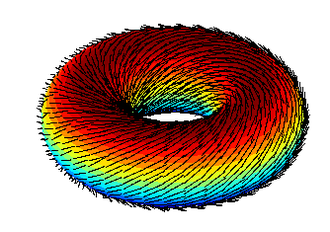
- Recall that a closed (no boundary) orientable surface is characterized by genus \(g\) (number of “handles”)
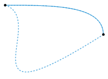
- For such a surface, there are \(2g\) closed curves, up to homotopy (see right), that generate all closed curves on the surface
- As an example, consider the torus, with the curves illustrated to the right.

Tree-Cotree for finding generators
- Build a spanning tree \(T^*\) of dual edges
- Build a spanning tree \(T\) of primary edges that doesn’t cross \(T^*\)
- There should be \(2g\) dual edges not contained in \(T^*\), and not crossed by \(T\)
- For each such edge, the corresponding generator is gotten by connecting the endpoints through \(T^*\)

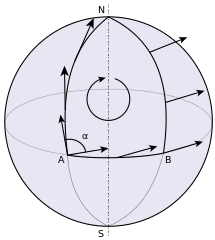
Levi-Civita Connections and Holonomy
- Primary question(s): how do you compare vectors in different tangent spaces? How can you transport vectors from one tangent space to another?
- A connection tells you how to do this. Levi-Civita connection is the canonical one.
- Allows one to differentiate one vector field \(\mathbf{w}\) with respect to another \(\mathbf{v}\).
- For an embedded surface: \(\nabla_\mathbf{v} \mathbf{w} = \mathrm{proj}_{T_\mathbf{p}\mathcal{S}} (\mathbf{w} \circ \alpha)'(0)\)
- One may also use it to parallel transport a vector along a curve.
- Holonomy associated with a path is the difference you get upon return.
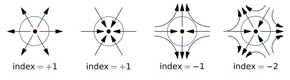
Poincare-Hopf Theorem
For a closed surface \(\mathcal{S}\) of genus \(g\), with a vector field \(\mathbf{v}\), with isolated zeros \(p_i\):
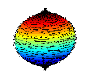
\[ \sum_{p_i} \mathrm{ind}_{p_i}(v) = \chi(\mathcal{S}) = 2-2g\] A popular folk theorem that results is the Hairy Ball Theorem. On the sphere, there are no non-vanishing vector fields.
Index of a vector field
The index describes the winding that occurs around the zeros. Specifically, as you walk around the zero, consider the map:
\[ x \mapsto \frac{\mathbf{v}(x)}{\lVert \mathbf{v}(x) \rVert}\]