Title
Geometry Processing
Geometry Representations
Computer Graphics & Geometry Processing
Zero set defines curve/surface
- Kernel of function \(F: \R^n \to \R\)
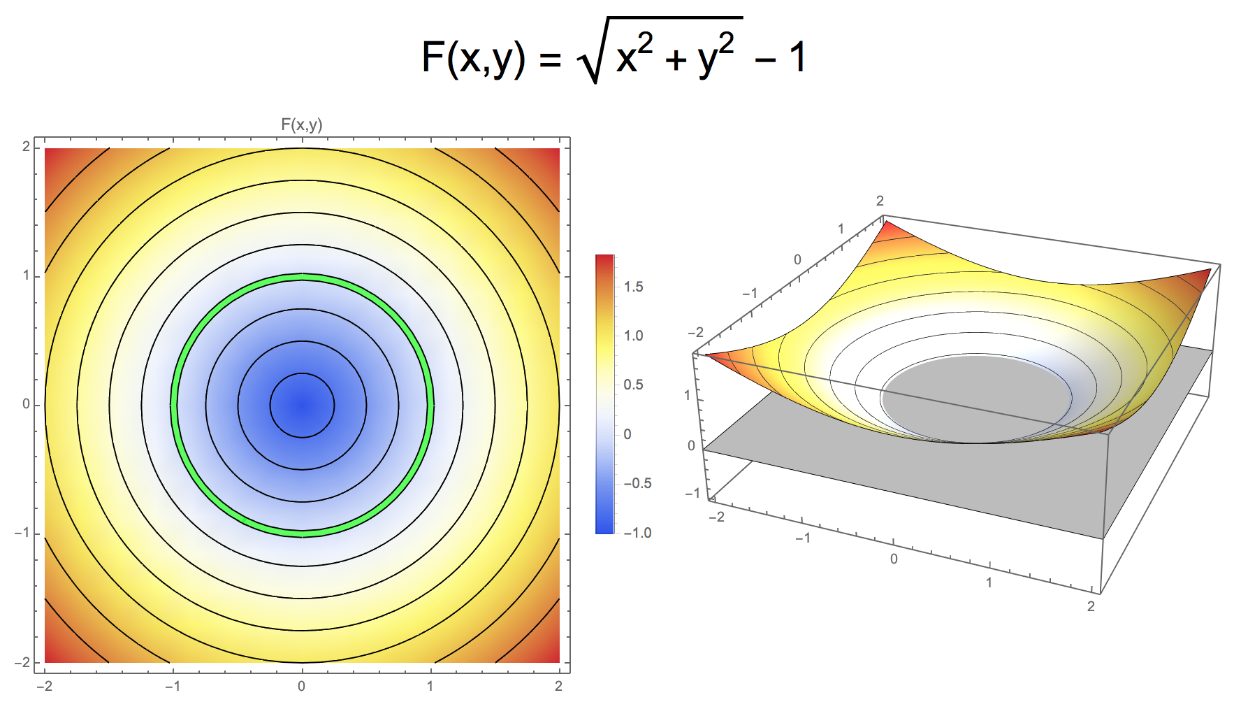
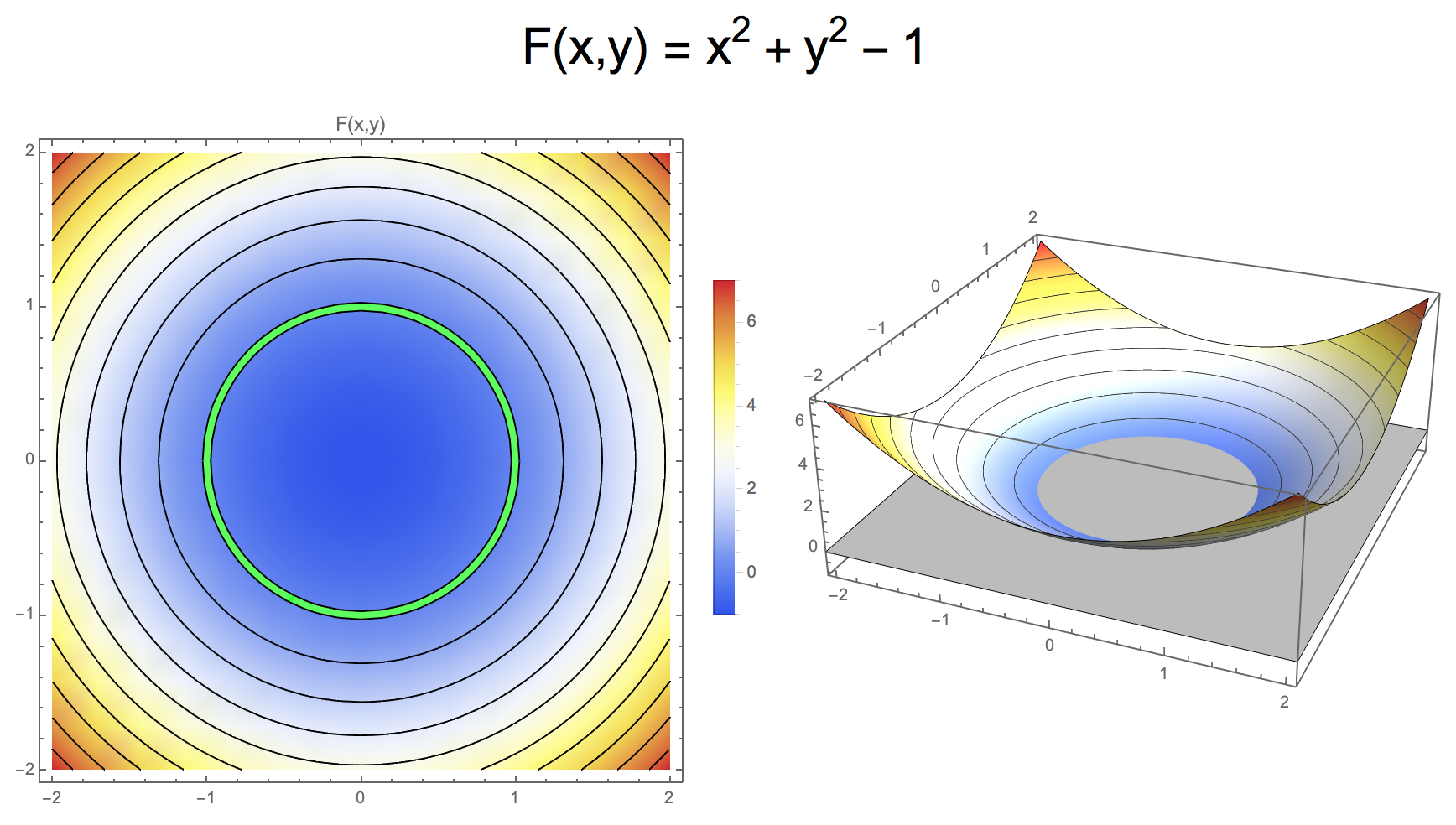
- Notion of distance not crucial, only zero set is relevant
- Different functions \(F\) can yield the same geometry
- Example: \(F(x,y) = \sqrt{x^2 + y^2} - 1\) or \(F(x,y) = x^2 + y^2 - 1\)
Gradient of Implicit Function
- Gradient of function \(F: \R^n \to \R\) is defined as \[\nabla F = \left[ \frac{\partial F}{\partial x_1},\, \frac{\partial F}{\partial x_2},\, \cdots,\, \frac{\partial F}{\partial x_n} \right]^T\]
Gradient of Implicit Function
- Gradient of function \(F: \R^n \to \R\) is defined as \[\nabla F = \left[ \frac{\partial F}{\partial x_1},\, \frac{\partial F}{\partial x_2},\, \cdots,\, \frac{\partial F}{\partial x_n} \right]^T\]
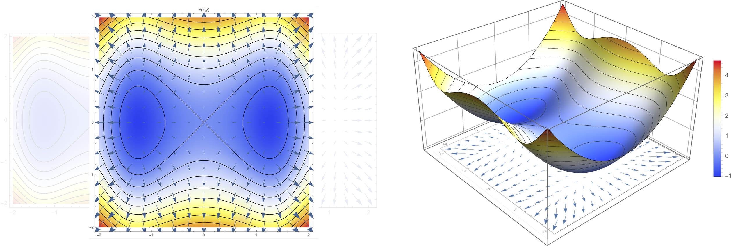
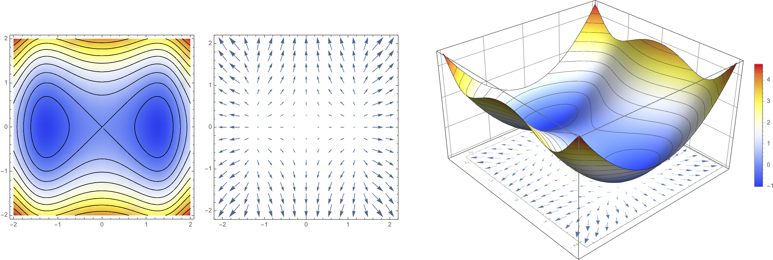
Gradient \(\nabla F\) is orthogonal to iso-surface
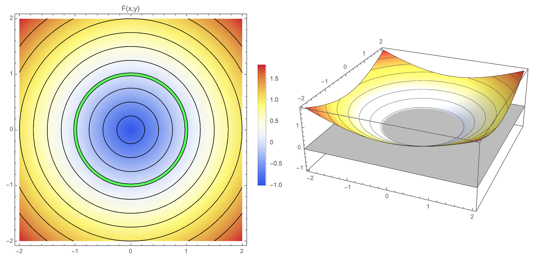
Signed Distance Function (SDF)
- Special case of an implicit representation
- \(F(\vec{x})\) gives signed distance to closest point on level surface
- Convention for sign: \(F(\vec{x}) < 0\) for interior, \(F(\vec{x}) > 0\) for exterior
- \(\nabla F\) is unit surface normal
- level sets are at constant offset distance
- SDF of circle: \[F(x,y) = \sqrt{x^2 + y^2} - 1\]
- SDF of sphere \[F(x,y,z) = \sqrt{x^2 + y^2 + z^2} - 1\]
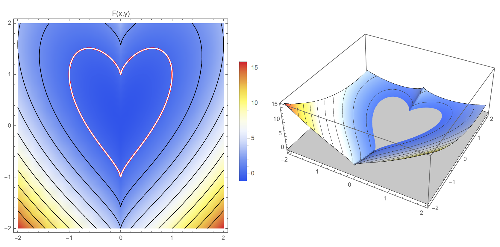
Modeling with Implicit Representations?
- Guess the shape of the curve! \[ F(x,y) = \left(y-\sqrt[3]{x^2}\right)^2 + x^2 - 1\]
Discrete Implicit Representation
- An implicit function \(F\) can be discretized by sampling
- Reconstruct continuous function from discrete values
- Example:
Discrete Implicit Representation
- An implicit function \(F\) can be discretized by sampling
- Reconstruct continuous function from discrete values
- Example: Piecewise linear representation on regular grid
2D Marching Squares Algorithm

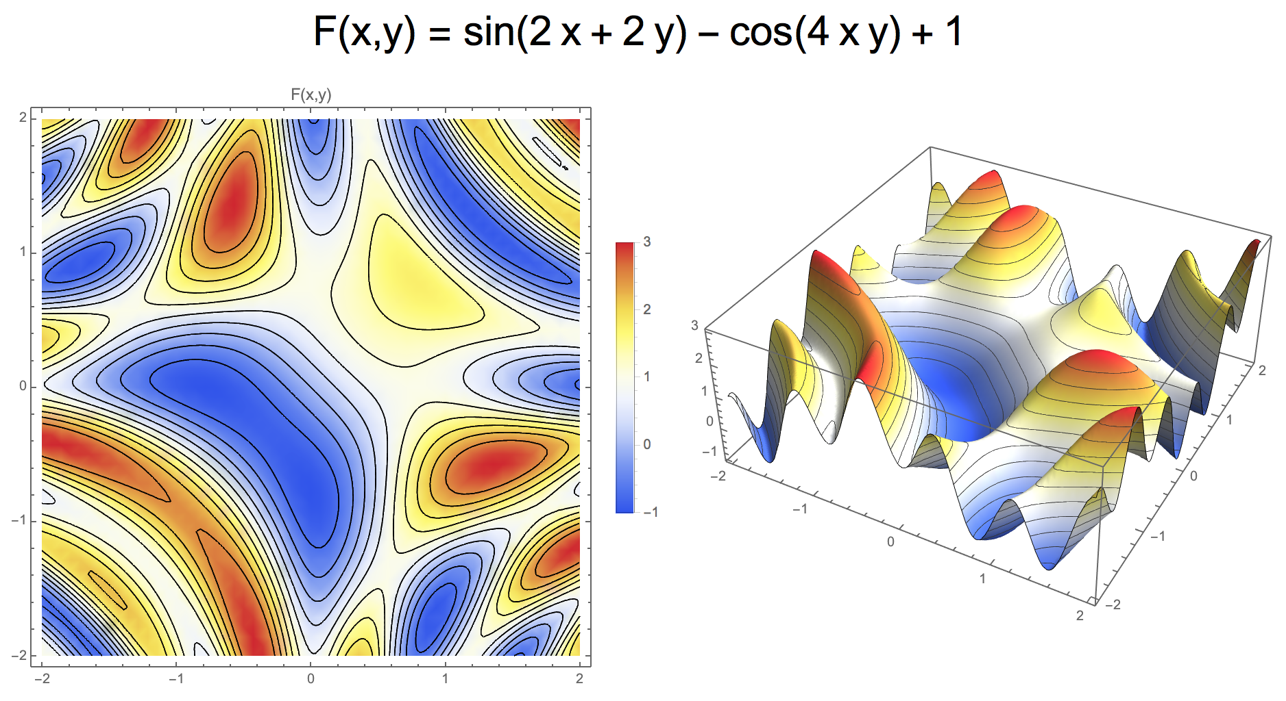
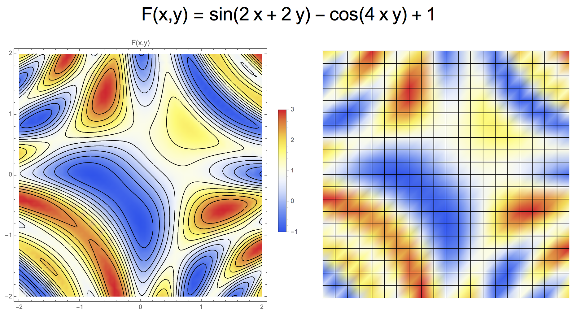
Application example
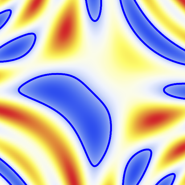
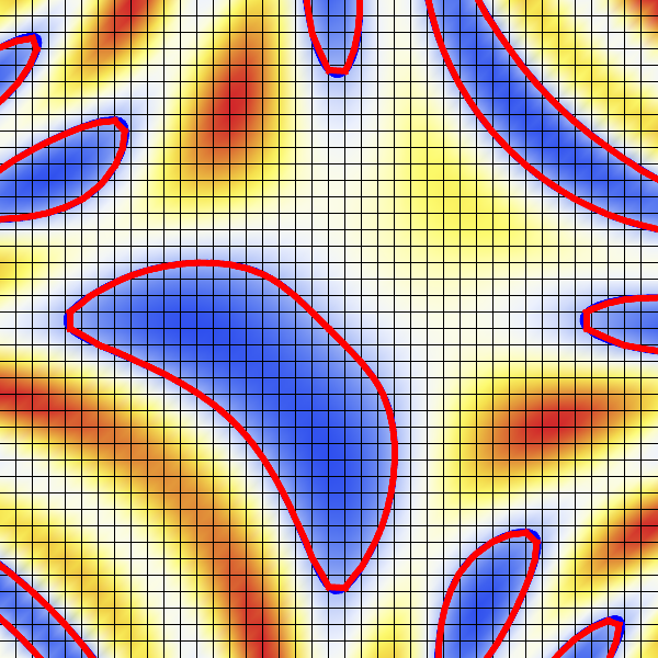
- Example: \(F(x,y)= \sin(2x + 2y) - \cos(4xy) + 1 = 0\)
- Increasing resolution reduces reconstruction error
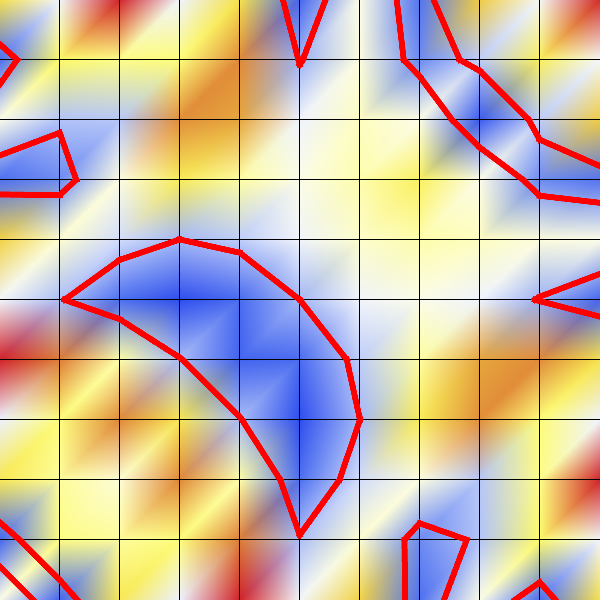
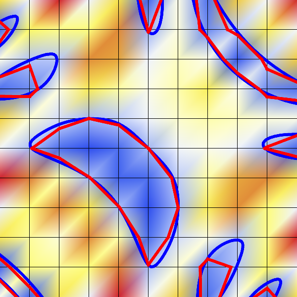
Application example
- Example: \(F(x,y)= \sin(2x + 2y) - \cos(4xy) + 1 = 0\)
- Increasing resolution reduces reconstruction error

3D Marching Cubes Algorithm
- Determine vertex positions
- linear interpolation of grid values along edges


3D Marching Cubes Algorithm
- Determine contour triangles
- look-up table for triangle configuration

3D Marching Cubes Algorithm

Parametric Representation
- Guess the shape of the curve! \[\vec{x}\of{t} = \matrix{\sin^3(t) \\ \frac{1}{16}(13\cos(t) - 5 \cos(2t) - 2 \cos(3t)-\cos(4t))}\]


Parametric Curve Properties
- A parametric curve \(\vec{x}\of{t}\) is
- simple: \(\vec{x}\of{t}\) is injective (no self-intersections)
- differentiable: \(\vec{x}’\of{t}\) is defined for all \(t \in [a,b]\)
- regular: \(\vec{x}’\of{t} \neq \vec{0}\) for all \(t \in [a,b]\)
- Which of the following are simple, differentiable, regular?


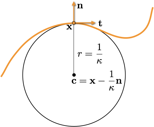
Curvature
- The osculating circle at point \(\vec{x}\) is the circle tangent to the curve at \(\vec{x}\) that best approximates the curve locally
(German: Schmiegkreis) - Its center is given as \(\vec{x} - \frac{1}{\kappa} \vec{n}\), where \(\kappa\) is the signed curvature and \(\vec{n}\) is the normal at \(\vec{x}\).
- Its radius is the inverse of the absolute curvature: \(r=1/|\kappa|\)