Infill Optimization for 3D printing
Wu et al., Infill Optimization for Additive Manufacturing, IEEE TVCG 2018.
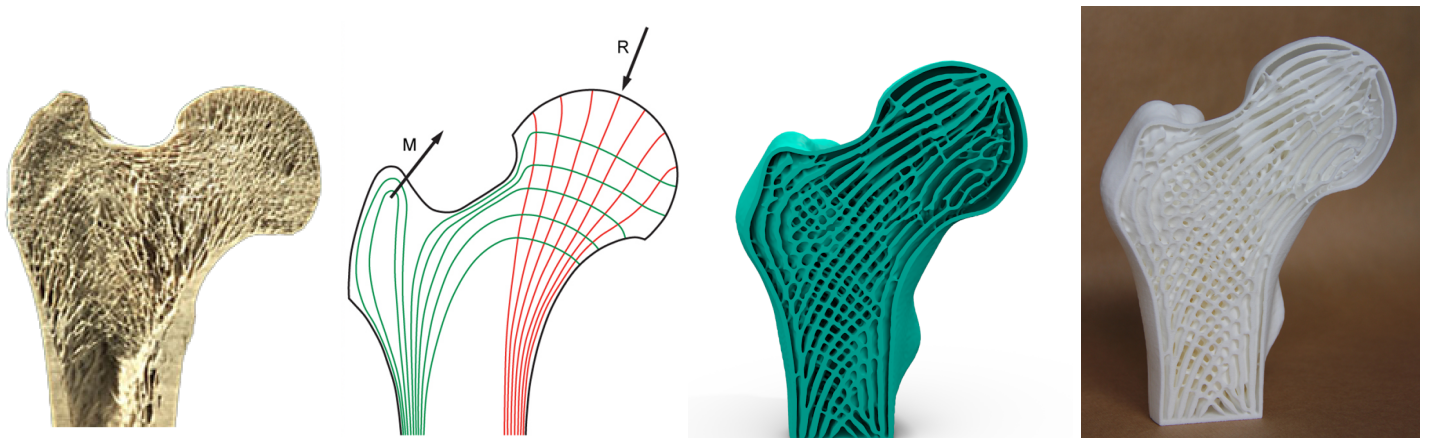
Infill Optimization for 3D printing
- Publicly available Matlab code!
- Simpler: Could apply to various models and load scenarios
- More difficult: Modify the method to optimize on different discretizations of the space

Stitch Meshing
Wu et al., Stitch Meshing, SIGGRAPH 2018

Again, code available! Similarly, one could look to apply it to models; or in a more difficult goal, try to allow user specification of singularities and defects.
Analytic Eigensystems for Distortion
Smith et al., Analytic Eigensystems for Isotropic Distortion Energies, SIGGRAPH 2018
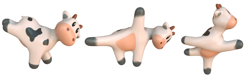
A project goal could be to implement the deformation model in 2D with the corresponding Projected Newton solver
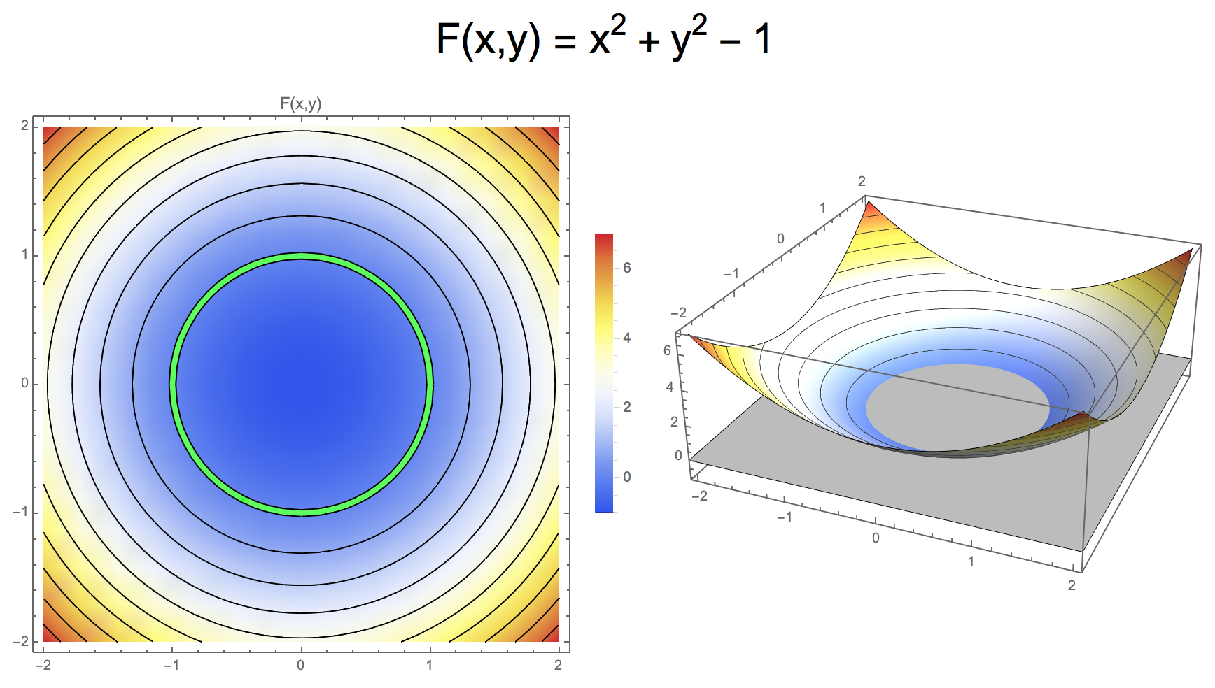
Zero set defines curve/surface
- Kernel of function \(F: \R^n \to \R\)
- Notion of distance not crucial, only zero set is relevant
- Different functions \(F\) can yield the same geometry
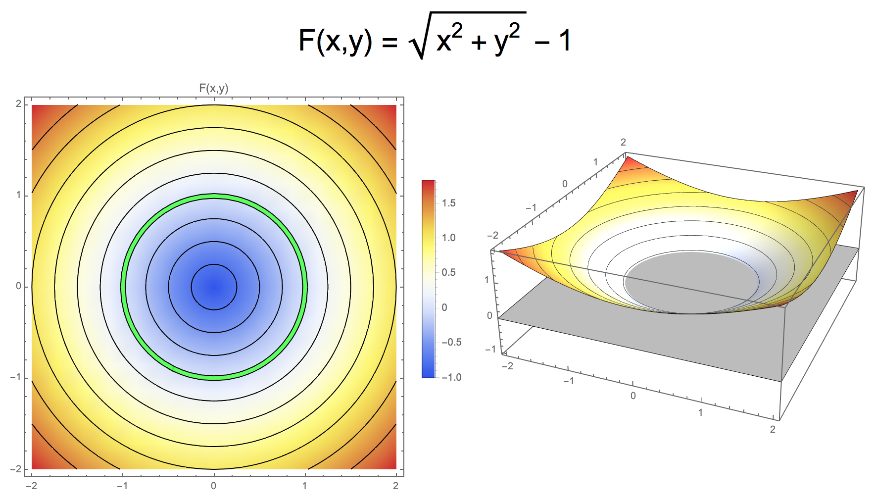
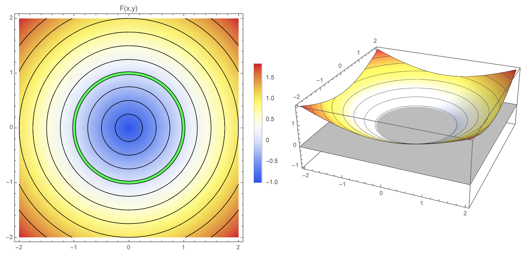
- Example: \(F(x,y) = \sqrt{x^2 + y^2} - 1\) or \(F(x,y) = x^2 + y^2 - 1\)
Gradient of Implicit Function
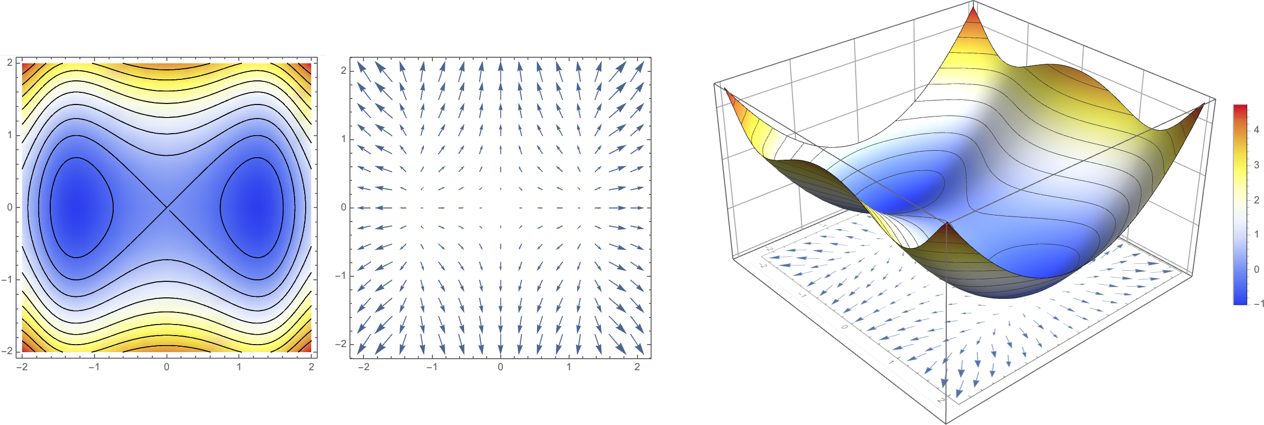
- Gradient of function \(F: \R^n \to \R\) is defined as \[\nabla F = \left[ \frac{\partial F}{\partial x_1},\, \frac{\partial F}{\partial x_2},\, \cdots,\, \frac{\partial F}{\partial x_n} \right]^T\]
Gradient of Implicit Function
- Gradient of function \(F: \R^n \to \R\) is defined as \[\nabla F = \left[ \frac{\partial F}{\partial x_1},\, \frac{\partial F}{\partial x_2},\, \cdots,\, \frac{\partial F}{\partial x_n} \right]^T\]
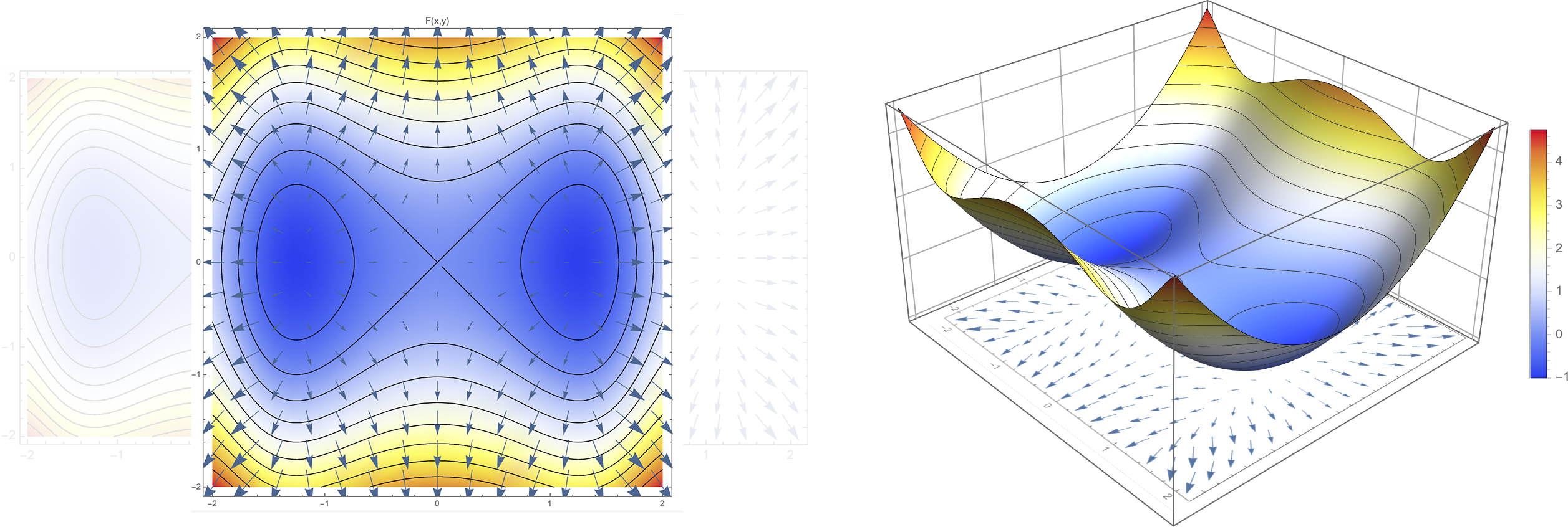
Gradient \(\nabla F\) is orthogonal to iso-surface
Signed Distance Function (SDF)
- Special case of an implicit representation
- \(F(\vec{x})\) gives signed distance to closest point on level surface
- Convention for sign: \(F(\vec{x}) < 0\) for interior, \(F(\vec{x}) > 0\) for exterior
- \(\nabla F\) is unit surface normal
- level sets are at constant offset distance
- SDF of circle: \[F(x,y) = \sqrt{x^2 + y^2} - 1\]
- SDF of sphere \[F(x,y,z) = \sqrt{x^2 + y^2 + z^2} - 1\]
Modeling with Implicit Representations?
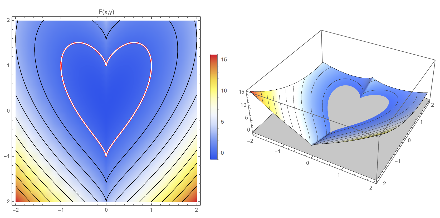
- Guess the shape of the curve! \[ F(x,y) = \left(y-\sqrt[3]{x^2}\right)^2 + x^2 - 1\]
Discrete Implicit Representation
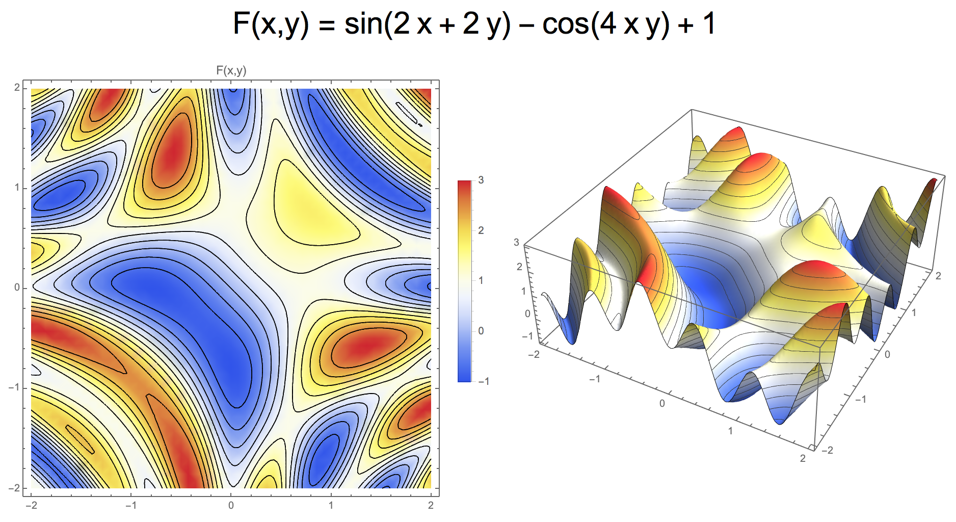
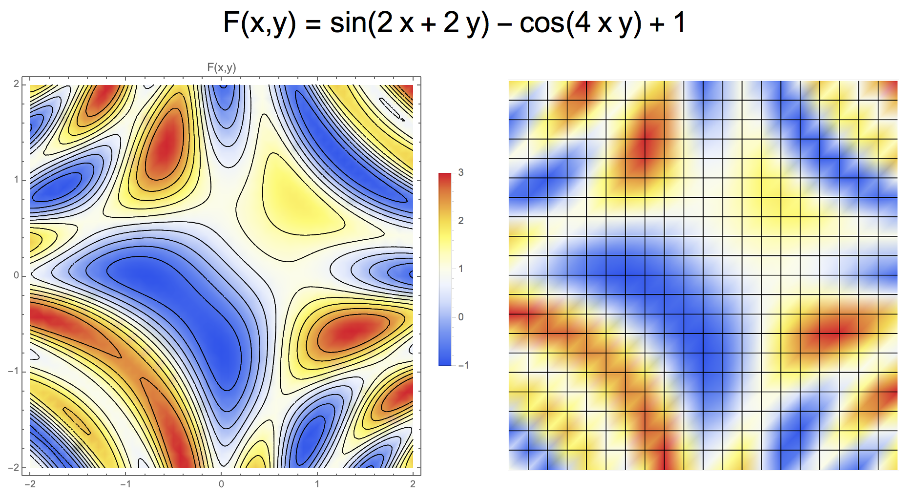
- An implicit function \(F\) can be discretized by sampling
- Reconstruct continuous function from discrete values
- Example:
Discrete Implicit Representation
- An implicit function \(F\) can be discretized by sampling
- Reconstruct continuous function from discrete values
- Example: Piecewise linear representation on regular grid
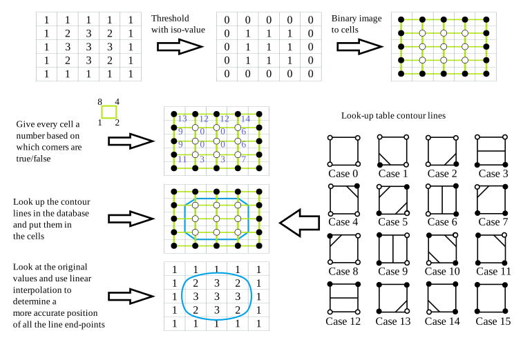
2D Marching Squares Algorithm
Application example
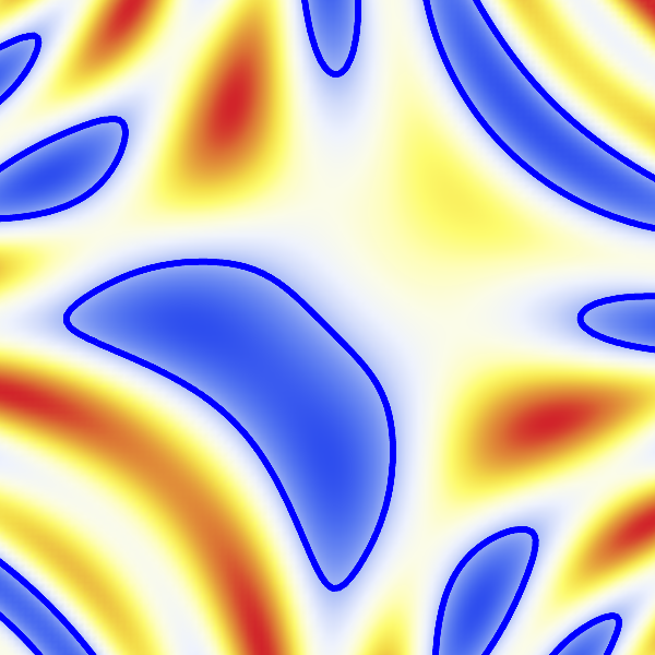
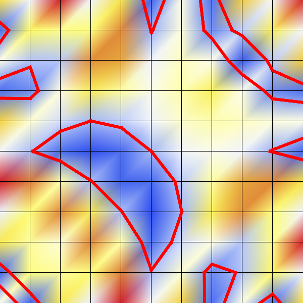
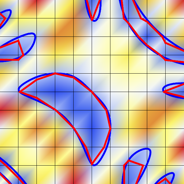
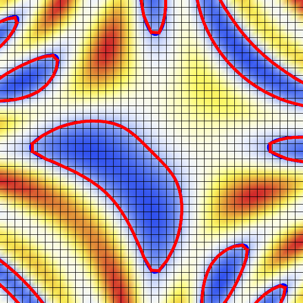
- Example: \(F(x,y)= \sin(2x + 2y) - \cos(4xy) + 1 = 0\)
- Increasing resolution reduces reconstruction error
Application example
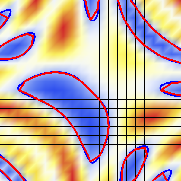
- Example: \(F(x,y)= \sin(2x + 2y) - \cos(4xy) + 1 = 0\)
- Increasing resolution reduces reconstruction error
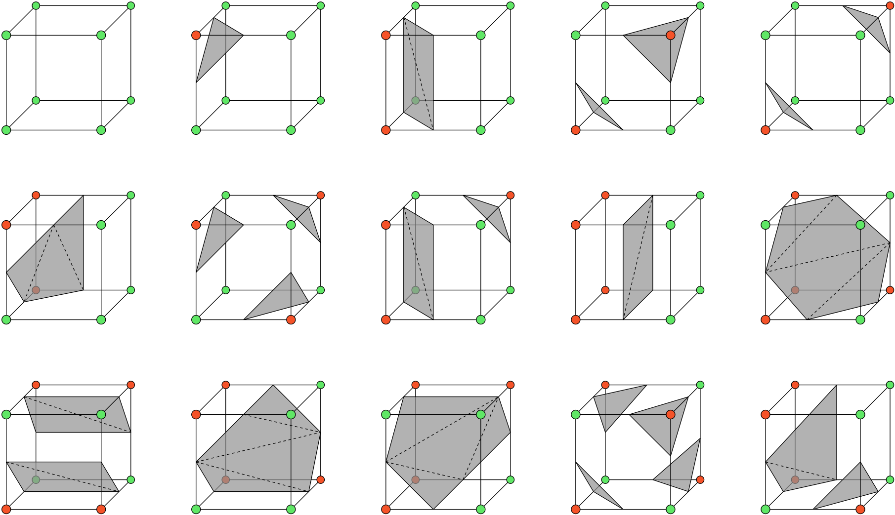
3D Marching Cubes Algorithm
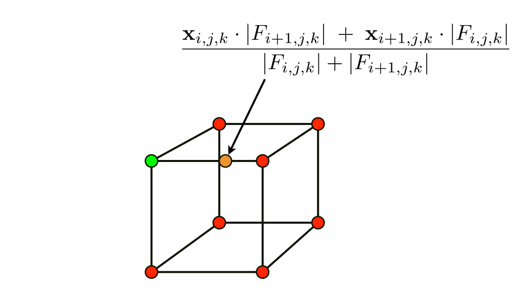
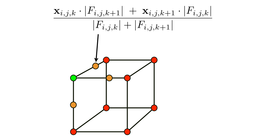
- Determine vertex positions
- linear interpolation of grid values along edges

3D Marching Cubes Algorithm
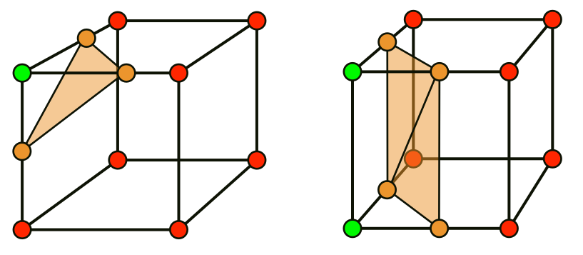
- Determine contour triangles
- look-up table for triangle configuration
3D Marching Cubes Algorithm
Parametric Representation
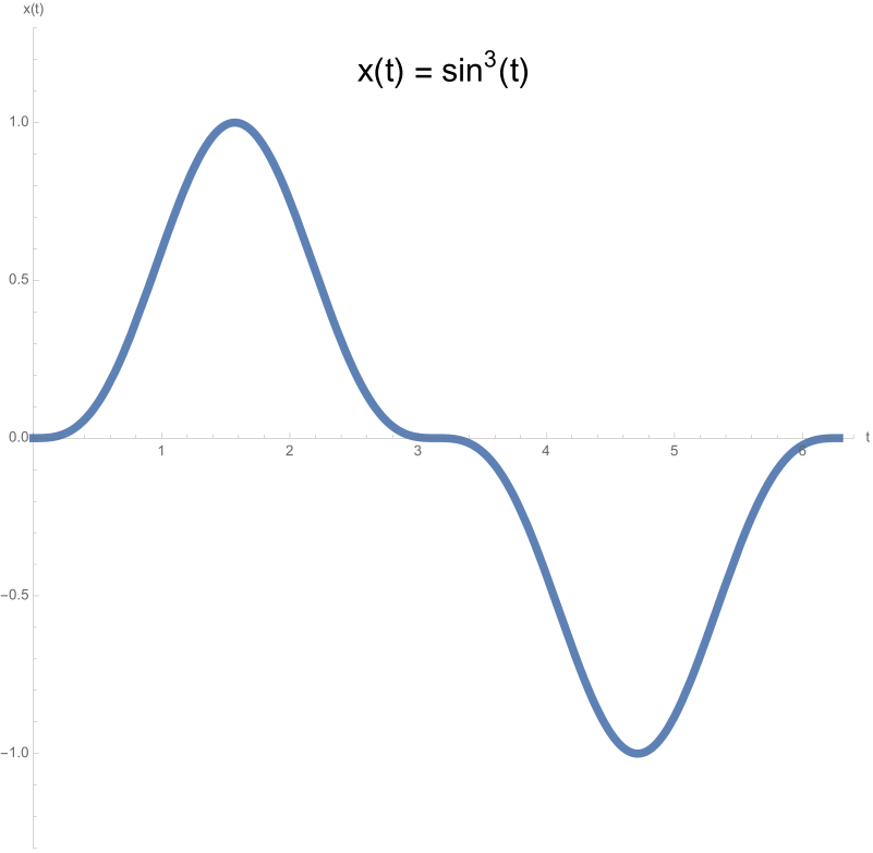
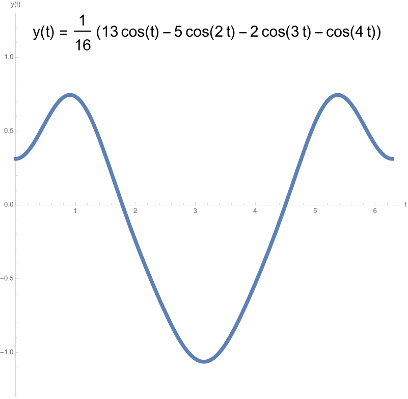
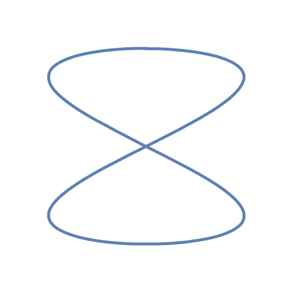
- Guess the shape of the curve! \[\vec{x}\of{t} = \matrix{\sin^3(t) \\ \frac{1}{16}(13\cos(t) - 5 \cos(2t) - 2 \cos(3t)-\cos(4t))}\]
Parametric Curve Properties
- A parametric curve \(\vec{x}\of{t}\) is
- simple: \(\vec{x}\of{t}\) is injective (no self-intersections)
- differentiable: \(\vec{x}’\of{t}\) is defined for all \(t \in [a,b]\)
- regular: \(\vec{x}’\of{t} \neq \vec{0}\) for all \(t \in [a,b]\)
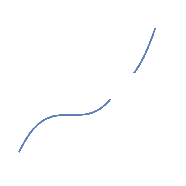
- Which of the following are simple, differentiable, regular?



Curvature
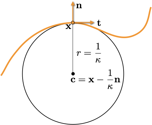
- The osculating circle at point \(\vec{x}\) is the circle tangent to the curve at \(\vec{x}\) that best approximates the curve locally
(German: Schmiegkreis) - Its center is given as \(\vec{x} - \frac{1}{\kappa} \vec{n}\), where \(\kappa\) is the signed curvature and \(\vec{n}\) is the normal at \(\vec{x}\).
- Its radius is the inverse of the absolute curvature: \(r=1/|\kappa|\)