Title
Arc Length Parameterization
- Intuitively, think about a rope of length \(L = \int \norm{\vec{x}’} \mathrm{d}t\) that is bend (but not stretched or compressed!) to assume the shape of the curve
- Curves parameterized with respect to arc length have some useful properties
- Unit speed: \(\norm{ \vec{x}'(s) } = 1\)
- Orthogonality: \(\vec{x}'(s) \cdot \vec{x}''(s) = 0\)
Gauss Map

Curvature
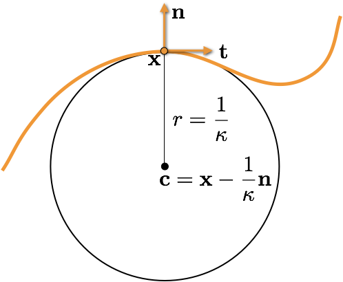
- The osculating circle at point \(\vec{x}\) is the circle tangent to the curve at \(\vec{x}\) that best approximates the curve locally
- Its center is given as \(\vec{x} + \frac{1}{\kappa} \vec{n}\), where \(\kappa\) is the signed curvature and \(\vec{n}\) is the normal at \(\vec{x}\).
- Its radius is the inverse of the absolute curvature, i.e. \(1/|\kappa|\)
A bit of info on 3D Curves
- For 3D curves \(\vec{x}: [a,b] \subset \R \mapsto \R^3\), there is another quantity to consider, that of torsion
\[\begin{aligned}{\dfrac {d\mathbf {T} }{ds}}&=\kappa \mathbf {N} ,\\{\dfrac {d\mathbf {N} }{ds}}&=-\kappa \mathbf {T} +\tau \mathbf {B} ,\\{\dfrac {d\mathbf {B} }{ds}}&=-\tau \mathbf {N} ,\end{aligned}\]
- Describes bending out of the plane
- Related work: Discrete Elastic Rods
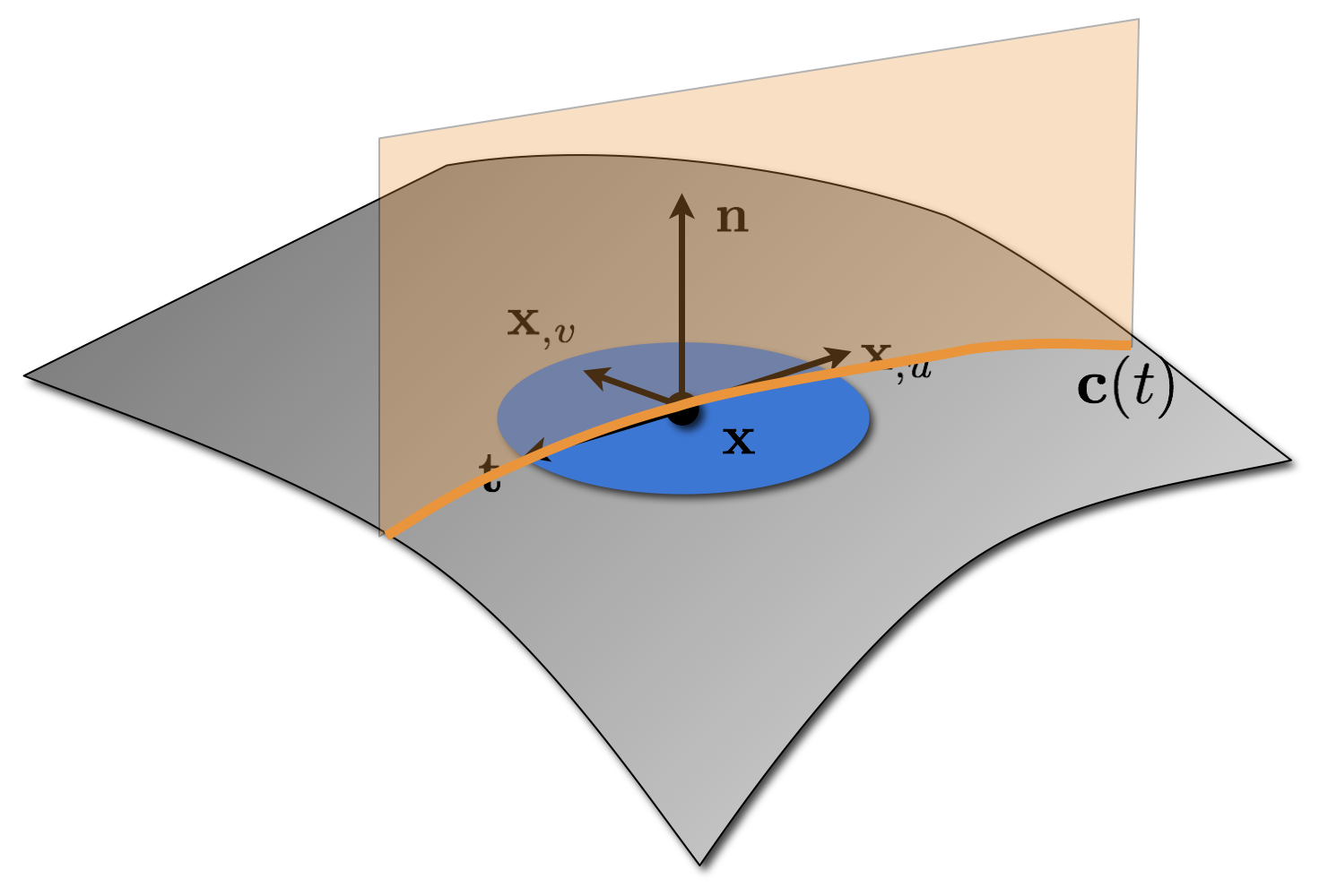
Curves on Surface
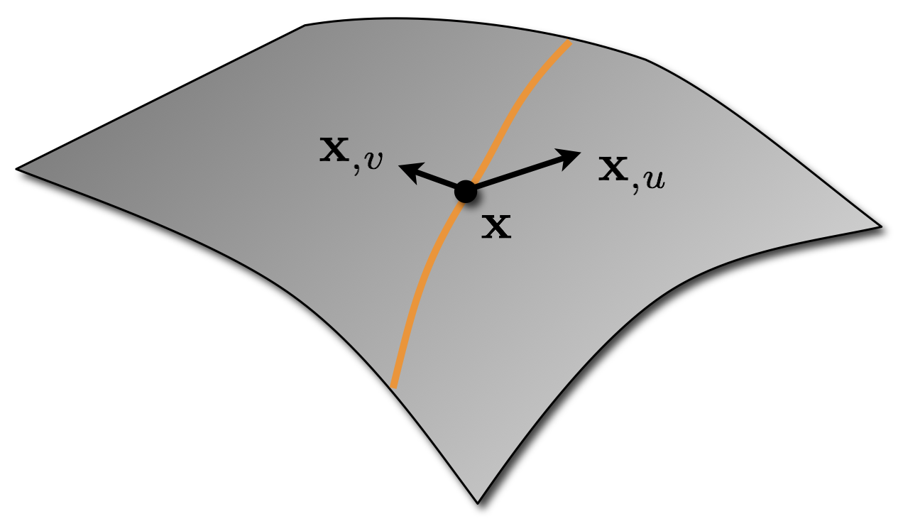
- A curve \((u(t), v(t))\) in the \(uv\)-plane defines a curve on the surface \(\vec{x}(u,v)\): \[\vec{x}\of{t} \;=\; \vec{x}\of{ u\of{t}, v\of{t} }\]
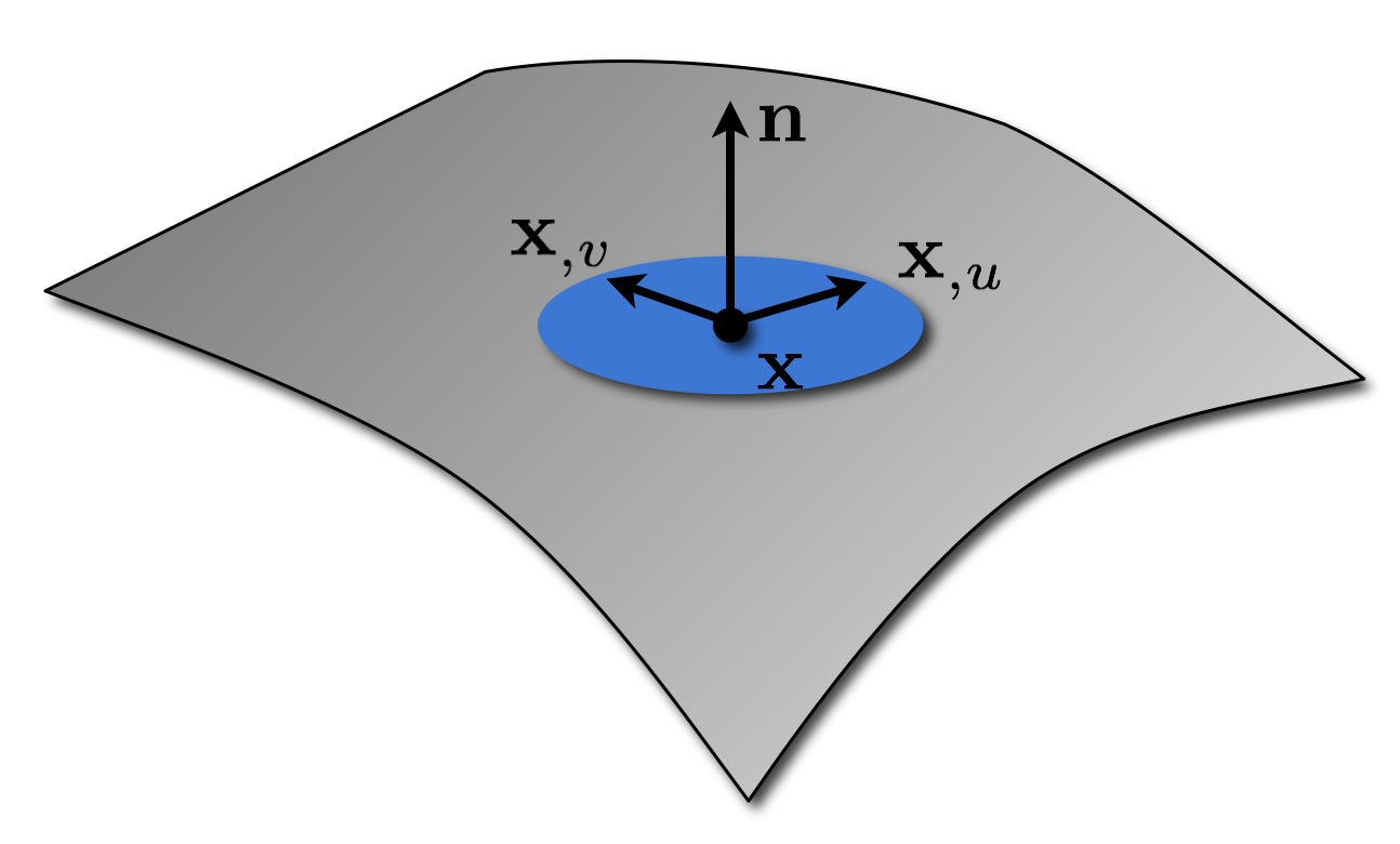
Parametric Surfaces
- Continuous surface \[\vec{x}\of{u,v} = \matrix{ x\of{u,v} \\ y\of{u,v} \\ z\of{u,v} }\]
- Normal vector \[\vec{n} = \frac{\vec{x}_{,u} \times \vec{x}_{,v}}{\norm{\vec{x}_{,u} \times \vec{x}_{,v}}}\]
- Assume regular parameterization \[\vec{x}_{,u} \times \vec{x}_{,v} \neq \vec{0}\]
Angles on Surface
- What is the angle of intersection of two curves \(\vec{c}_1\) and \(\vec{c}_2\) intersecting at \(\vec{x}\)?
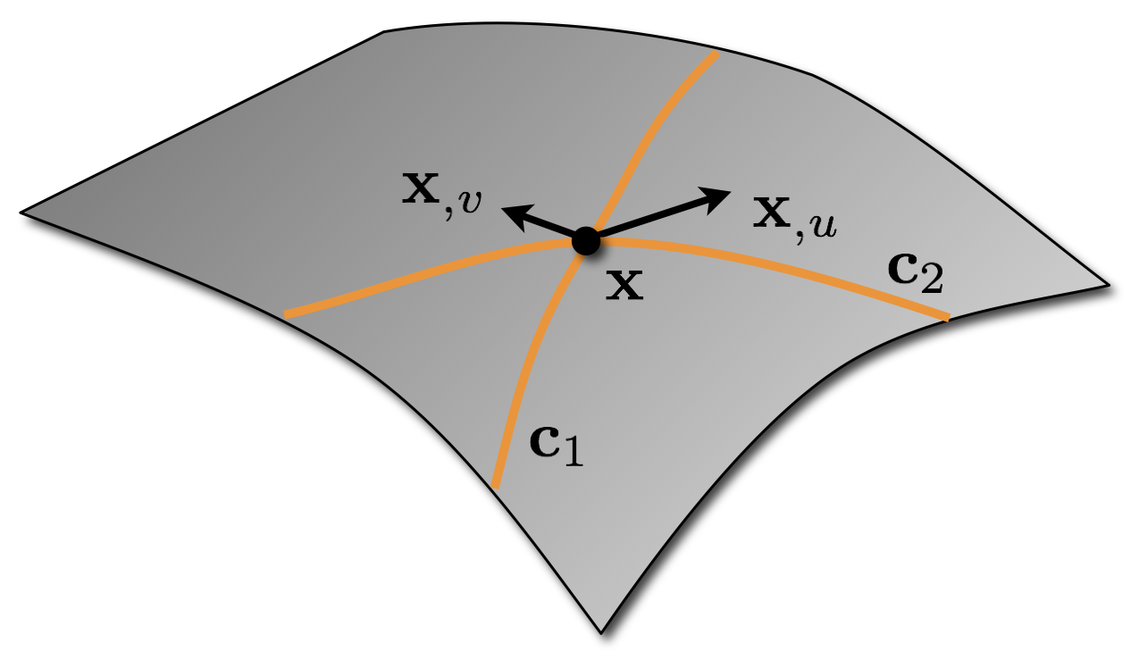
- Two tangents \(\vec{t}_1\) and \(\vec{t}_2\) \[ \vec{t}_i = \alpha_i \vec{x}_{,u} + \beta_i \vec{x}_{,v} \]
- Compute inner product \[ \begin{align} \trans{\vec{t}_1} \vec{t}_2 \;&=\; \cos\theta \norm{\vec{t}_1} \norm{\vec{t}_2} \\ \;&=\; \trans{\left(\alpha_1 \vec{x}_{,u} + \beta_1 \vec{x}_{,v} \right)} \left(\alpha_2 \vec{x}_{,u} + \beta_2 \vec{x}_{,v} \right) \\ \;&=\; \left( \alpha_1, \beta_1 \right) \matrix{ \trans{\vec{x}_{,u}} \vec{x}_{,u} & \trans{\vec{x}_{,u}} \vec{x}_{,v} \\[1mm] \trans{\vec{x}_{,u}} \vec{x}_{,v} & \trans{\vec{x}_{,v}} \vec{x}_{,v} } \matrix{\alpha_2 \\ \beta_2 } \end{align} \]
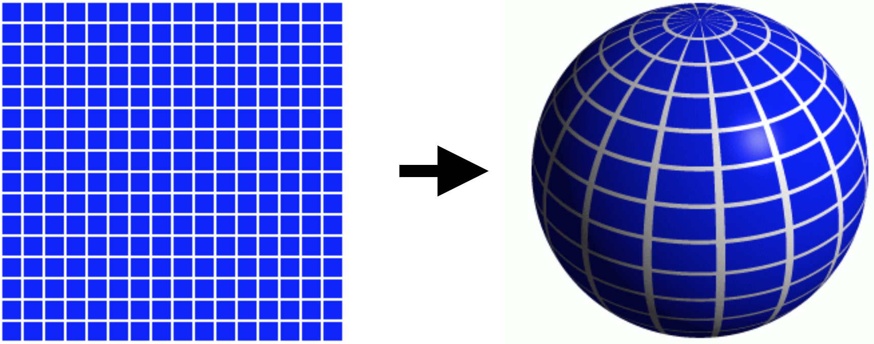
Example: Unit Sphere
- Spherical parameterization
\[\vec{x}\of{u,v} \;=\; \matrix{\cos u \sin v \\ \sin u \sin v \\ \cos v} \,,\quad (u,v) \in [0, 2\pi) \times [0,\pi) \]
Example: Unit Sphere
- Length of equator \(\vec{x}(t, \pi / 2)\)
- \(u(t)=t\) and \(u'(t)=1\)
- \(v(t)=\pi/2\) and \(v'(t)=0\)
\[ \begin{align} \int_0^{2\pi} 1 \,\func{d}s \;&=\; \int_0^{2\pi} \sqrt{E \, u_{,t}^2 + 2F \, u_{,t} v_{,t} + G \, v_{,t}^2} \,\func{d}t \\ \;&=\; \int_0^{2\pi} \sin v \,\func{d}t \\ \;&=\; 2\pi \sin v \;=\; 2\pi \end{align} \]
Example: Unit Sphere
- Area of sphere
\[ \begin{align} \int_0^{\pi}\int_0^{2\pi} 1 \,\func{d}A \;&=\; \int_0^{\pi}\int_0^{2\pi} \sqrt{EG-F^2} \,\func{d}u\,\func{d}v \\ \;&=\; \int_0^{\pi}\int_0^{2\pi} \sin v \,\func{d}u\,\func{d}v \\ \;&=\; 4\pi \end{align} \]
Normal Curvature
- Let \(\vec{t}\) be a tangent vector at \(\vec{x}\).
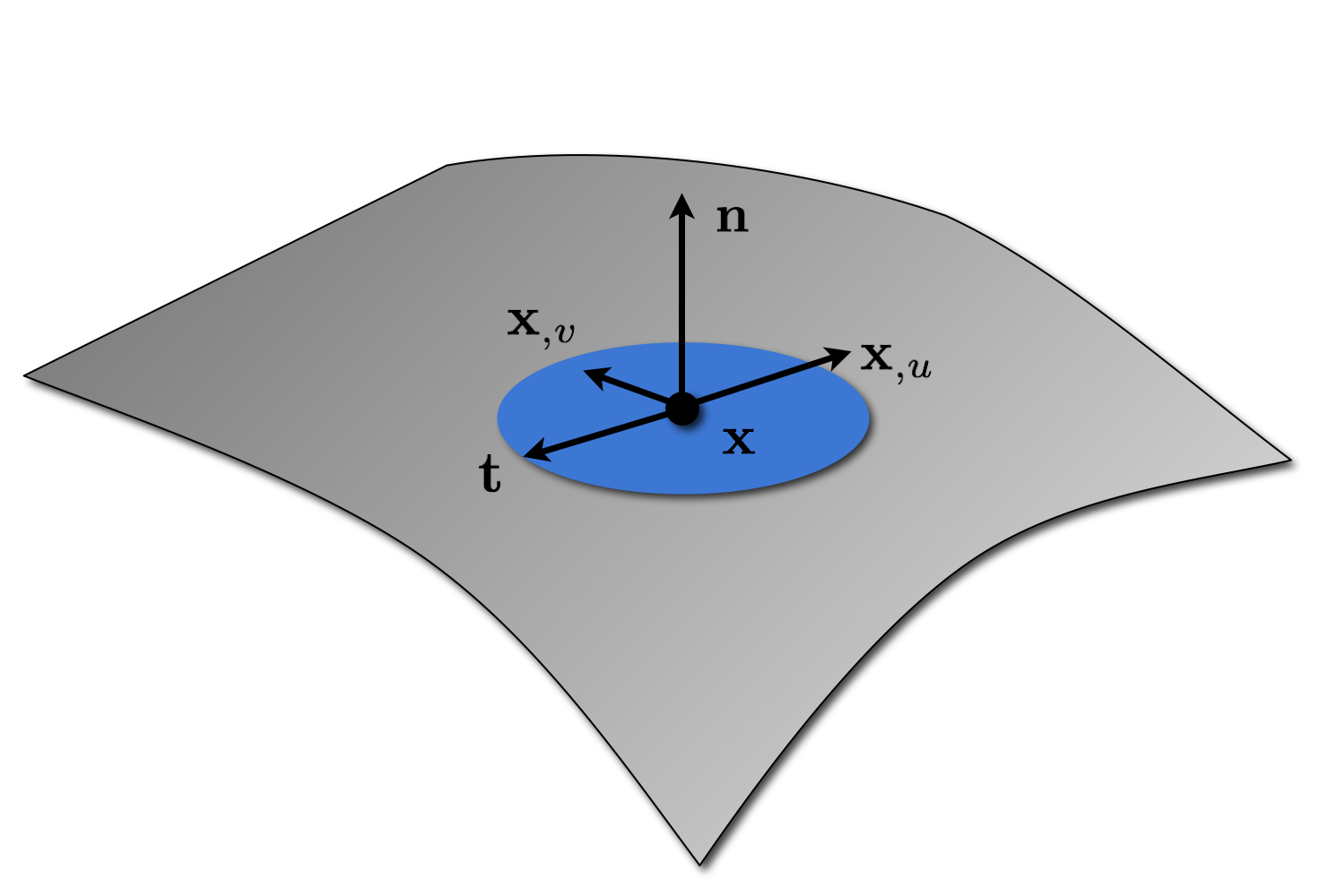
Normal Curvature
- Let \(\vec{t}\) be a tangent vector at \(\vec{x}\).
- \(\vec{x}\), \(\vec{n}\), and \(\vec{t}\) define a normal plane. The intersection of this plane with the surface yields a curve \(\vec{x}(t)\), called a normal section.
Normal Curvature
- Let \(\vec{t}(\phi) = \cos \phi \vec{x}_{,u} + \sin \phi \vec{x}_{,v}\) be a tangent vector at \(\vec{x}\) and assume that \(\vec{x}_{,u}\) and \(\vec{x}_{,v}\) are orthonormal.
- We can plot \(\kappa_n(\vec{t}(\phi))\) as a function of the tangent angle \(\phi\)
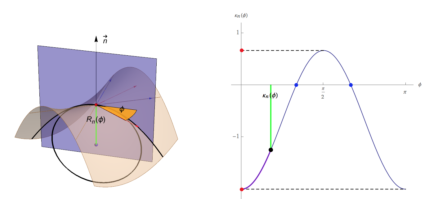
Surface Curvature(s)
- Principal curvatures
- Maximum curvature \(\kappa_1 = \max_{\phi} \kappa_n(\phi)\)
- Minimum curvature \(\kappa_2 = \min_{\phi} \kappa_n(\phi)\)
- Euler theorem: \(\kappa_n\of{\phi} \;=\; \kappa_1\cos^2\phi + \kappa_2\sin^2\phi\)
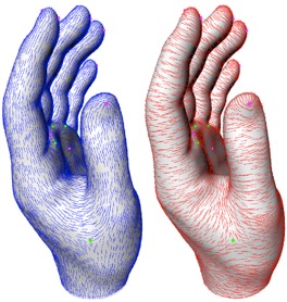
- Corresponding principal directions \(\vec{e}_1\), \(\vec{e}_2\) are orthogonal
- Maximum curvature \(\kappa_1 = \max_{\phi} \kappa_n(\phi)\)
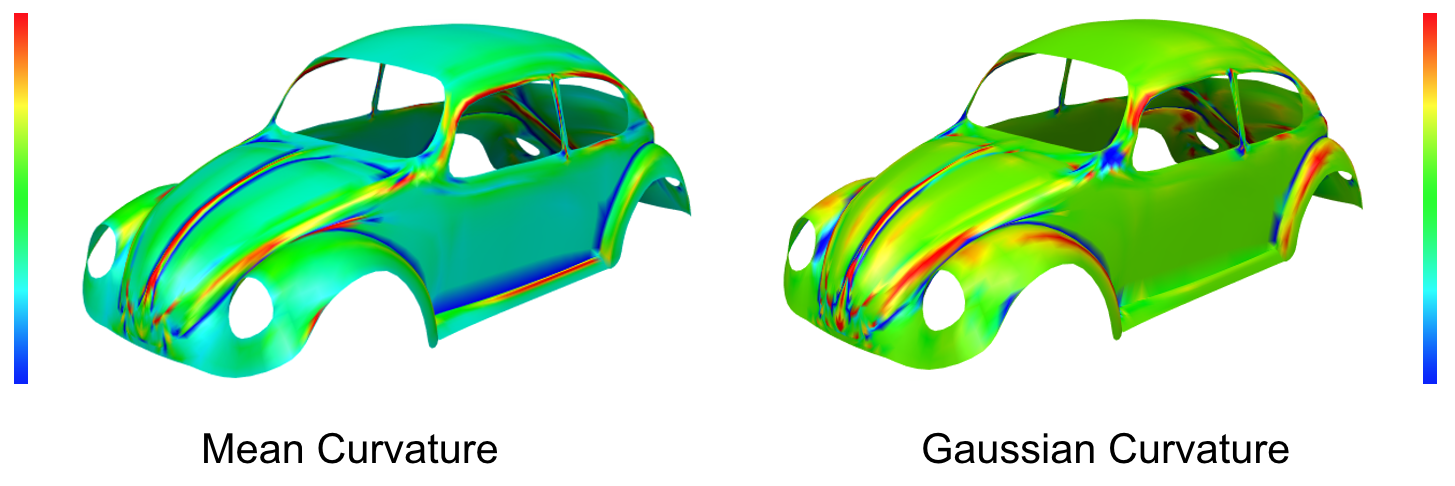
Surface Curvature(s)
- Special curvatures
- Mean curvature \(H= \frac{1}{2\pi} \int_0^{2 \pi} \kappa_n(\phi) \text{d} \phi = \frac{\kappa_1+\kappa_2}{2}\)
- Gaussian curvature \(K = \kappa_1 \cdot \kappa_2\)
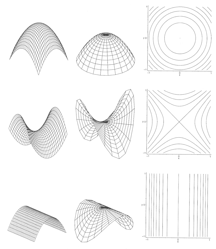
Classification
A point \(\vec{x}\) on the surface is called
- elliptic, if \(K > 0\)
- hyperbolic, if \(K < 0\)
- parabolic, if \(K = 0\)
- umbilic, if \(\kappa_1 = \kappa_2\)
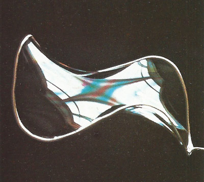
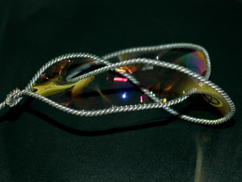
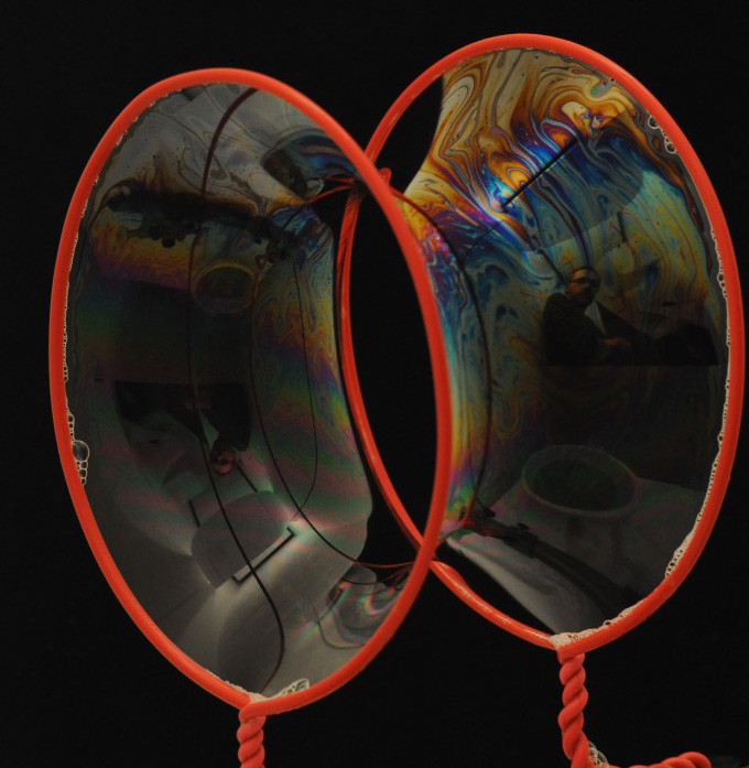
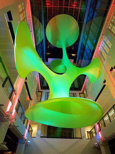
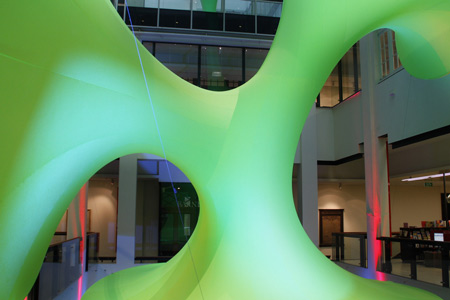
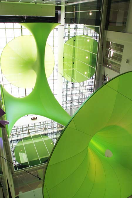
Minimal Surfaces
- Mean curvature \(H = \frac{\kappa_1 + \kappa_2}{2}\)
- \(H = 0\) everywhere → minimal surface
- all points must be hyperbolic (saddle points)
- Example: Soap films

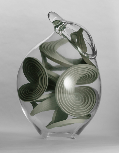
Minimal Surfaces
- Mean curvature \(H = \frac{\kappa_1 + \kappa_2}{2}\)
- \(H = 0\) everywhere → minimal surface
- all points must be hyperbolic (saddle points)
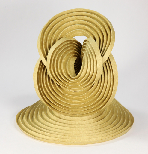
- Example: Sculpture
Developable Surfaces
- Gaussian curvature \(K = \kappa_1 \cdot \kappa_2\)
- \(K = 0\) everywhere → developable surface
- all points must be parabolic
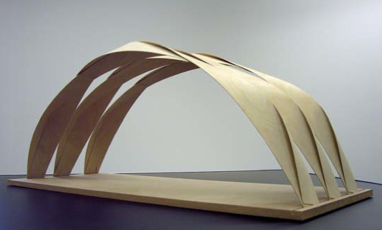
Developable Surfaces
- Curved foldings
Recap: Differential Operators
- Gradient \(\begin{eqnarray*} \nabla f := \left(\frac{\partial f}{\partial x_1}, \ldots, \frac{\partial f}{\partial x_n} \right) \end{eqnarray*}\)
- points in direction of steepest ascent
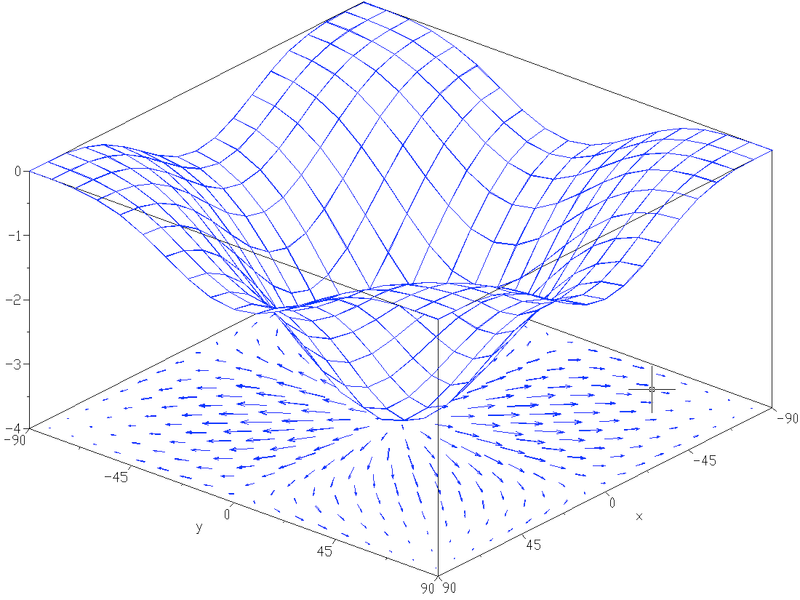
Recap: Differential Operators
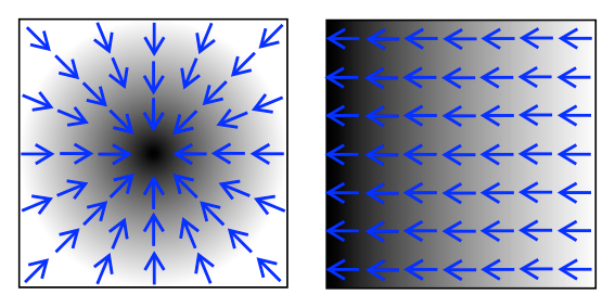
- Divergence \(\begin{eqnarray*} \text{div} F = \nabla \cdot F := \frac{\partial F_1}{\partial x_1} + \ldots + \frac{\partial F_n}{\partial x_n} \end{eqnarray*}\)
- volume density of outward flux of vector field
- magnitude of source or sink at given point
