Title
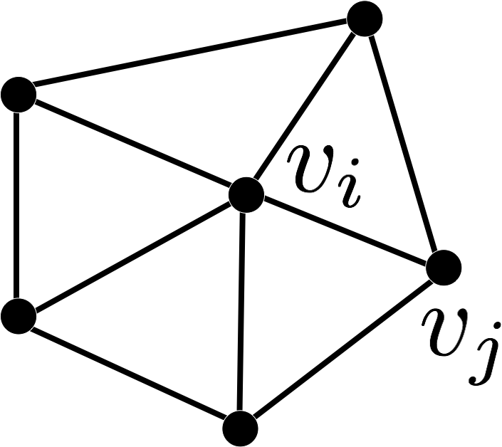
Uniform Laplace
- Uniform Laplace-Beltrami discretization \[ \laplace f\of{v_i} \;:=\; \frac{1}{\abs{\set{N}_1\of{v_i}}} \sum_{v_j \in \set{N}_1\of{v_i}} \left( f\of{v_j} - f\of{v_i} \right) \]
- Properties
- depends only on connectivity
- does not take into account geometry at all
- not accurate for irregular triangulations
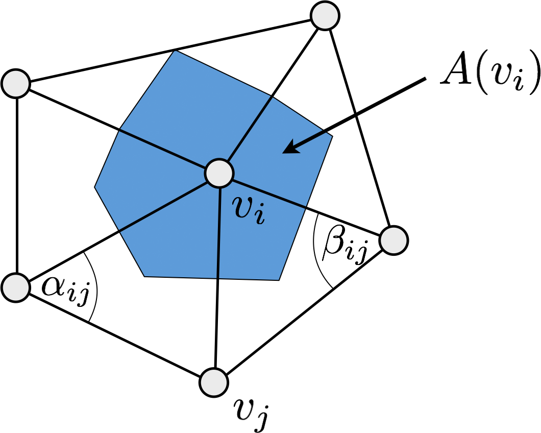
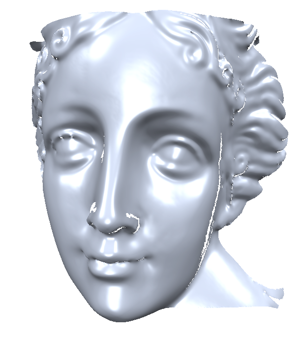
Discrete Laplace-Beltrami
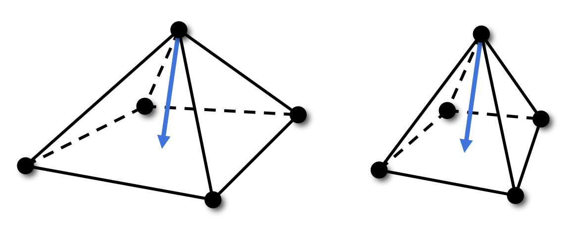
- Cotangent Laplace-Beltrami discretization \[ \laplace_{\set{S}} f\of{v_i} \;:=\; \frac{1}{2A\of{v_i}} \sum_{v_j \in \set{N}_1\of{v_i}} \left( \cot \alpha_{ij} + \cot \beta_{ij} \right) \left( f\of{v_j} - f\of{v_i} \right)\]
- Properties
- depends on connectivity and geometry
- more accurate than uniform discretization
- weights can become negative
- most frequently used discretization
Motivation
- Filter out high-frequency noise
Motivation
- Filter out high-frequency noise
Motivation
- Advanced filtering
Fourier Transform
- Represent a function as a weighted sum of sine and cosine functions
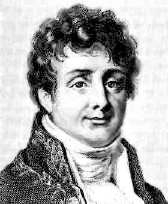
(1768-1830)
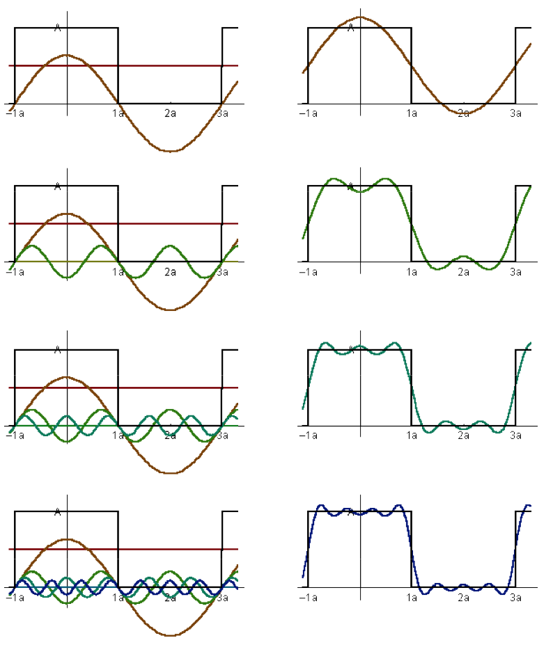
\[ f\of{x} \;=\; a_0 + a_1 \cos\of{x} + a_2 \cos\of{3x} + a_3 \cos\of{5x} + a_4 \cos\of{7x} + \dots \]
Fourier Transform
\[F(\omega) = \int_{-\infty}^{\infty} f(x) \, \func{e}^{-2\pi\func{i}\omega x} \func{d}x\]
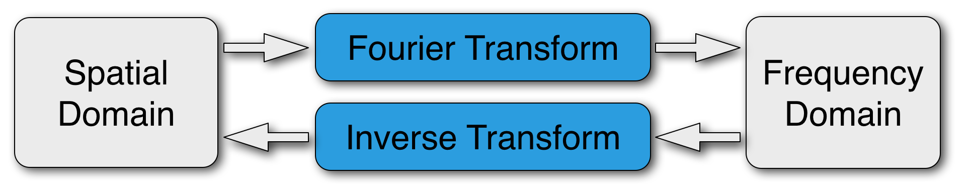
\[f(x) = \int_{-\infty}^{\infty} F(\omega) \, \func{e}^{2\pi\func{i}\omega x} \;\func{d}\omega\]
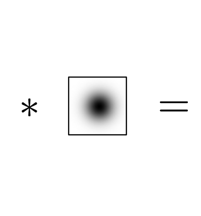
Convolution
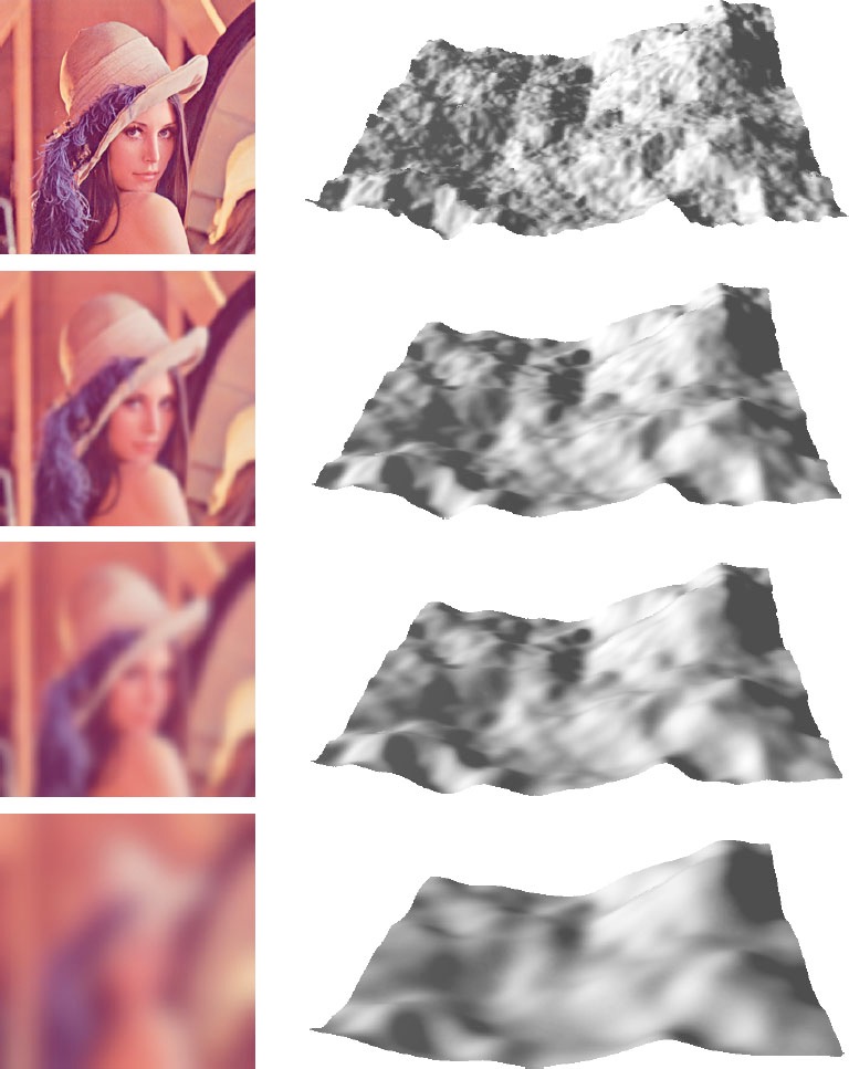
Smooth signal by convolution with a kernel function \[ h(x) \;=\; f * g \;:=\; \int f(y) \cdot g(x-y) \,\func{d}y \]
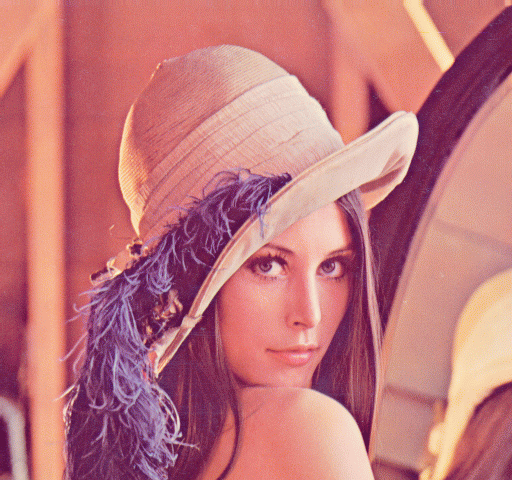
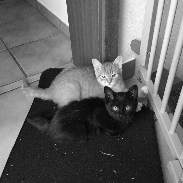
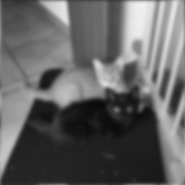
Example: Gaussian blurring
![lenna.png]()
![lenna_equation.png]()
![lenna_smooth.png]()

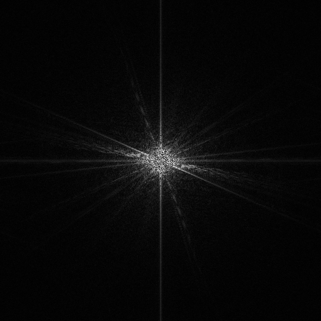
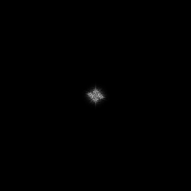
Filtering with Fourier Transform


Filtering with Fourier Transform
Discrete Laplace-Beltrami
- Function values sampled at the \(n\) mesh vertices \[\vec{f} = [f(v_1), f(v_2), \ldots, f(v_n)]\T \in \R^n\]
- Discrete Laplace-Beltrami (per vertex) \[ \laplace f\of{v_i} = \frac{1}{2A_i} \sum_{v_j \in \set{N}_1\of{v_i}} \left( \func{cot} \alpha_{ij} + \func{cot} \beta_{ij} \right) \left( f \of{v_j} - f \of{v_i} \right)\]
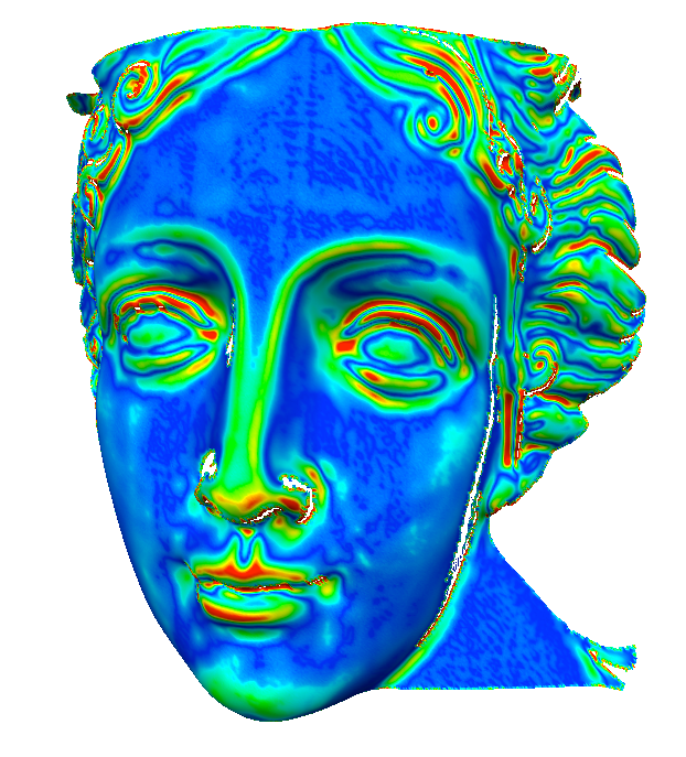
Spectral Mesh Analysis
- Discrete Laplace operator is sparse matrix \(\mat{L} = \mat{DM} \in \R^{n \times n}\)
- Eigenvectors are “natural vibrations”
- Eigenvalues are “natural frequencies”
Levy, Zhang: Spectral Mesh Processing, SIGGRAPH Courses 2010
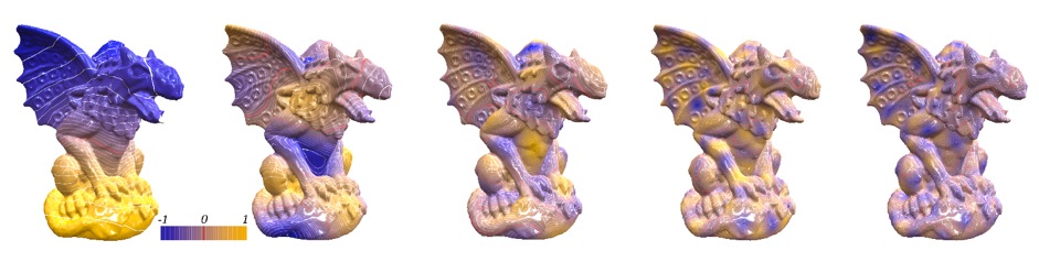
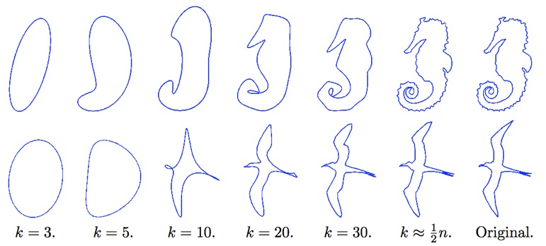
Spectral Mesh Analysis
- Setup Laplace-Beltrami matrix \(\vec{L}\)
- Compute \(k\) smallest eigenvectors \(\{\vec{e}_1, \ldots, \vec{e}_k\}\)
- Reconstruct mesh from those (component-wise)
Levy, Zhang: Spectral Mesh Processing, SIGGRAPH Courses 2010
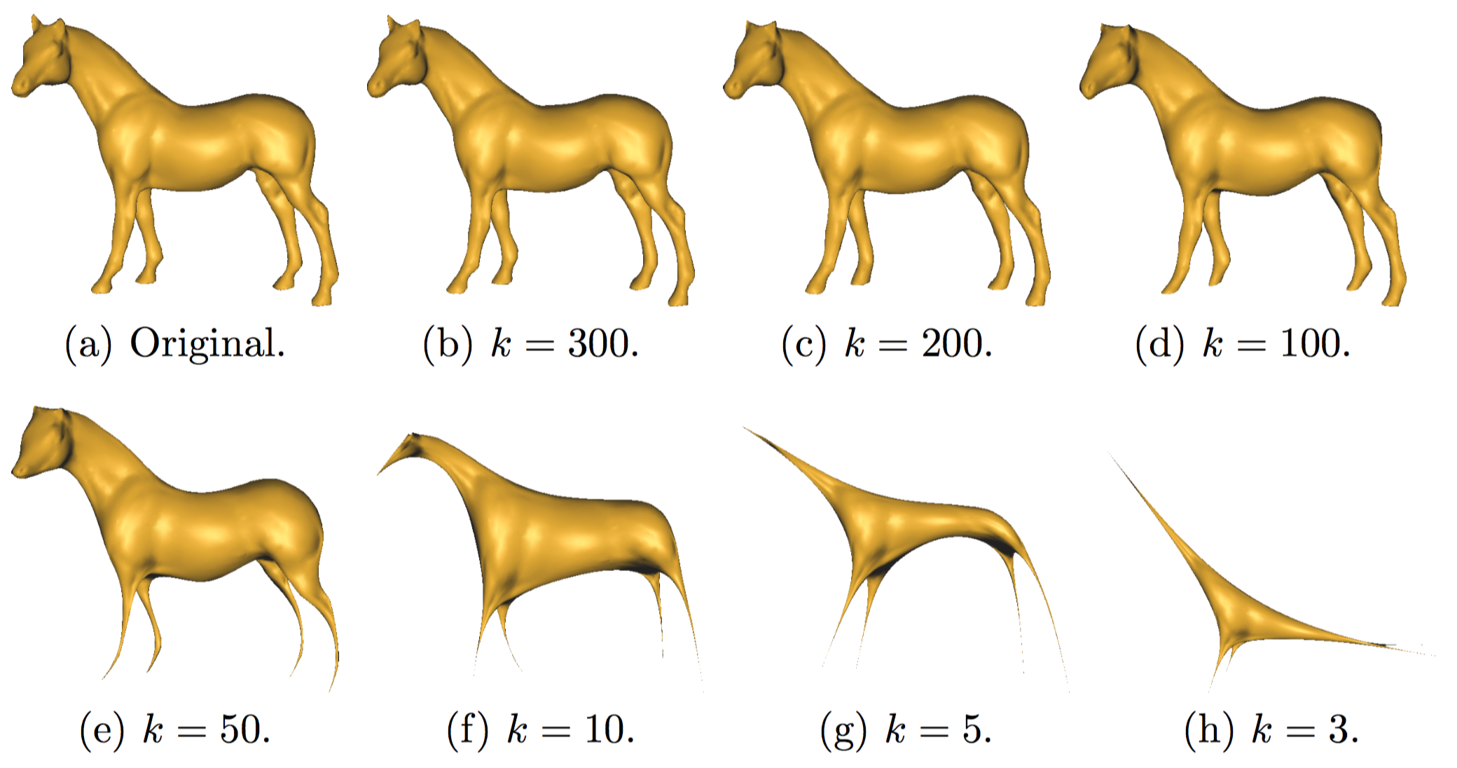
Spectral Mesh Analysis
- Setup Laplace-Beltrami matrix \(\vec{L}\)
- Compute \(k\) smallest eigenvectors \(\{\vec{e}_1, \ldots, \vec{e}_k\}\) Too complex for large meshes 😢
- Reconstruct mesh from those (component-wise)
Levy, Zhang: Spectral Mesh Processing, SIGGRAPH Courses 2010
Diffusion Flow
- Diffusion equation is frequently used to smooth signals \[\frac{\partial f}{\partial t} = \lambda \Delta f\]
- \(\lambda\) is the diffusion constant
- \(\Delta\) is the Laplace operator
- Solve numerically
- Discretize function in space & time
- Discretize time derivative
- Discretize spatial derivatives
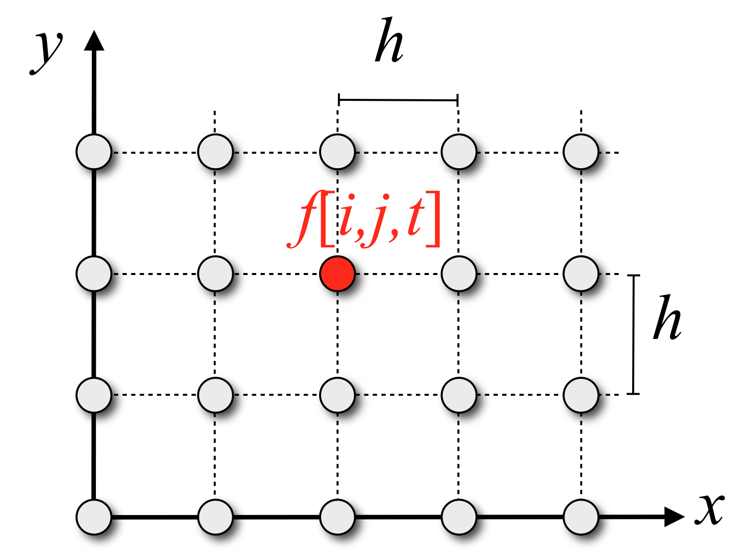
Discretize PDE on Regular Grid
- Sample function \(f(x,y,t)\) on a regular grid with spacing \(h\) and time-step \(\delta_t\) \[f[i,j,t] \;=\; f\left(i \cdot h, j \cdot h, t \cdot \delta t \right) \]
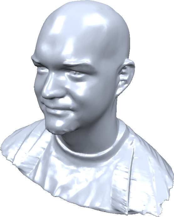
Diffusion Flow on Meshes
- Continuous PDE: \(\frac{\partial \vec{x}}{\partial t} \;=\; \lambda \Delta \vec{x}\)
- Discretization: \(\vec{x}_i \leftarrow \vec{x}_i + \delta t \, \lambda \Delta \vec{x}_i\)
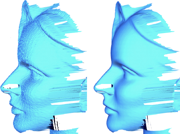
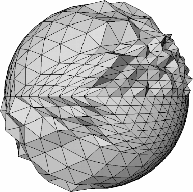
Uniform Laplace Discretization
- Smoothes geometry and triangulation
- Can be non-zero even for planar triangulations
- Vertex drift can lead to distortions
- Might be desired for mesh regularization
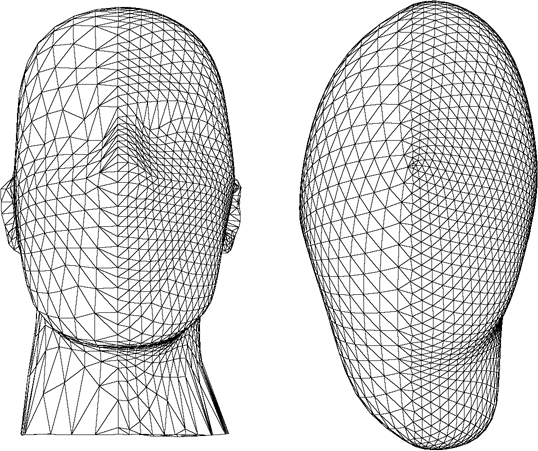
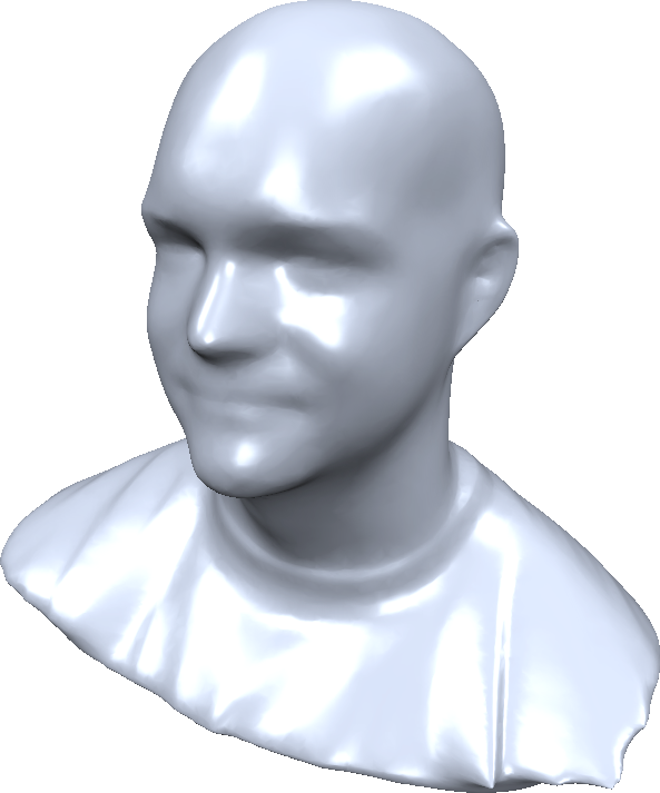
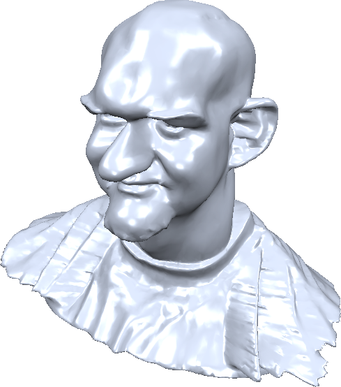
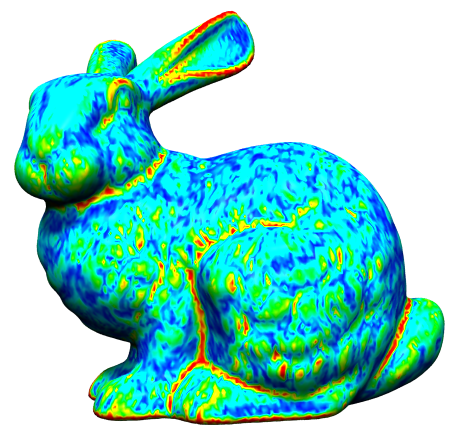
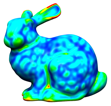
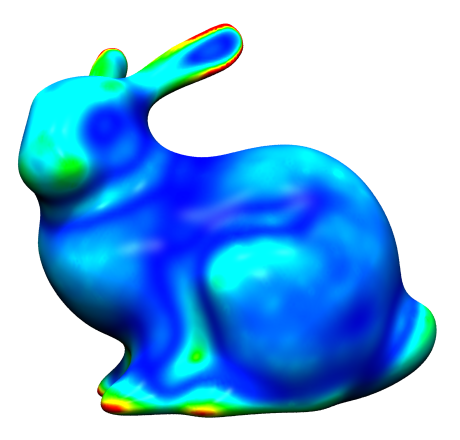
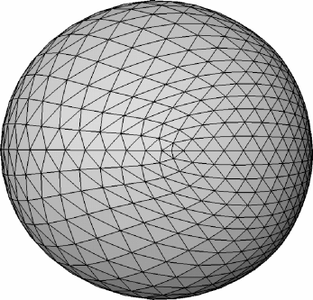
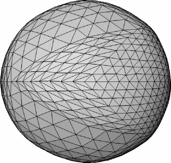
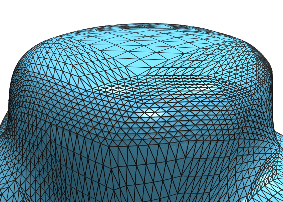
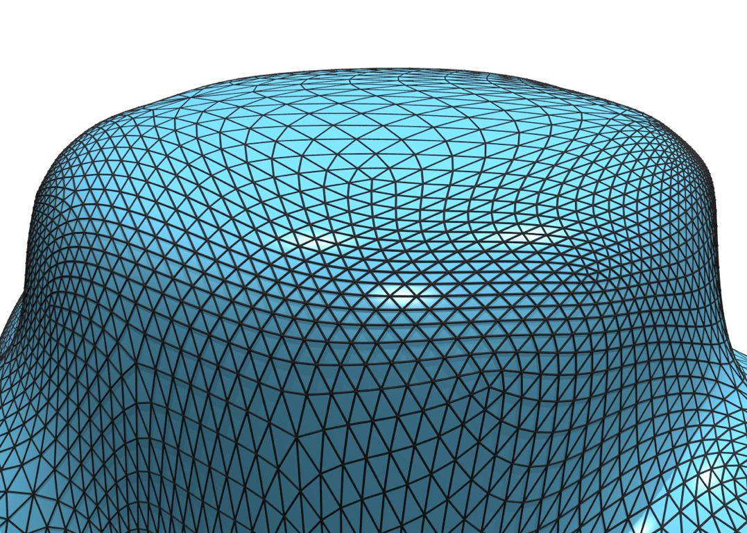
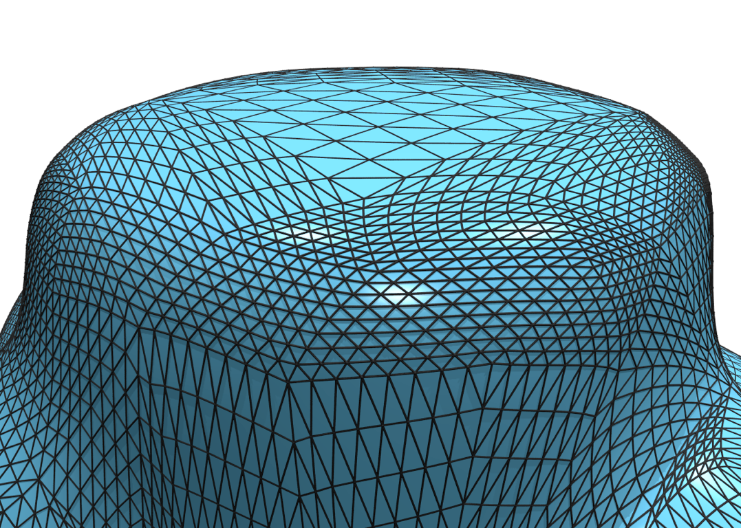
Uniform vs Cotan Discretization
How to solve the linear system?
- Solve linear system in each iteration \[(\vec{I} - \delta t \, \lambda \vec{L}) \vec{X}^{(t+1)} = \vec{X}^{(t)}\]
- Matrix \(\vec{L} = \vec{DM}\) is built from Laplace weights \[\mat{M}_{ij} \;=\; \begin{cases} \func{cot}\alpha_{ij} + \func{cot}\beta_{ij}, & i \ne j \,,\; j \in \set{N}_1\of{v_i} \\ - \sum_{v_j \in \set{N}_1 \of{v_i}}\of{ \func{cot}\alpha_{ij} + \func{cot}\beta_{ij} } & i=j \\ 0 & \text{otherwise} \end{cases} \]
\[\mat{D} = \func{diag}\of{ \dots, \frac{1}{2A_i}, \dots}\]
Literature
- Botsch et al., Polygon Mesh Processing, AK Peters, 2010
- Chapter 4
- Taubin, A Signal Processing Approach to Fair Surface Design, SIGGRAPH 1995
- Desbrun, Meyer, Schröder, Barr, Implicit Fairing of Irregular Meshes using Diffusion and Curvature Flow, SIGGRAPH 1999