Title
Geometry Processing
Delaunay Mesh Generation
Computer Graphics & Geometry Processing
Definition
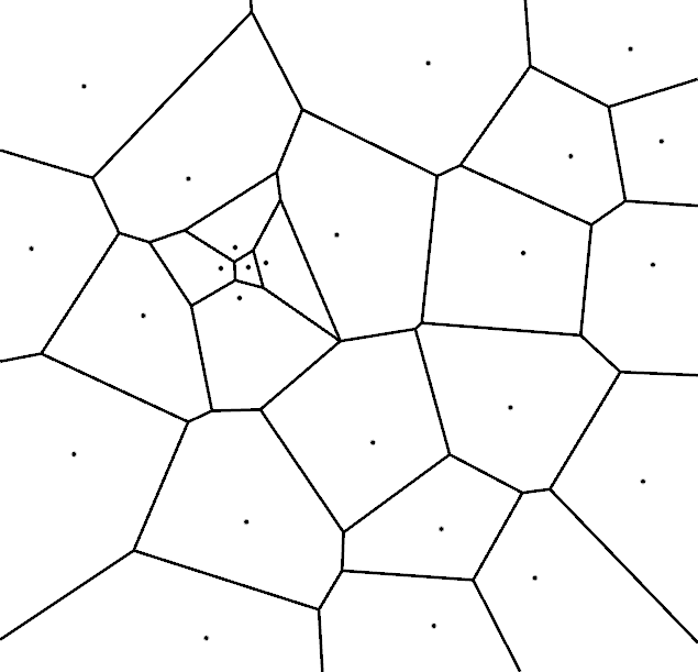
- Given a set of 2D sample points \(\{\vec{p}_1, \ldots, \vec{p}_n\}\)
- Partition the plane by assigning each 2D point \(\vec{x}\) to its nearest sample.
- All points assigned to \(\vec{p}_i\) form its Voronoi cell \[\set{V}(\vec{p}_i) = \left\{ \vec{x} \in \R^2: \norm{\vec{x}-\vec{p}_i} \leq \norm{\vec{x}-\vec{p}_j}, \; \forall j \neq i \right\}\]
- Edges and vertices of these cells form the Voronoi diagram (VD).
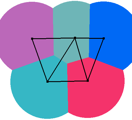
Voronoi Diagram


Voronoi Diagram
- Each point pair \(\vec{p}_i\), \(\vec{p}_j\) defines a perpendicular bisector
- The bisector of \(\vec{p}_i\) and \(\vec{p}_j\) defines two half-planes
- Let \(H(\vec{p}_i, \vec{p}_j)\) be the half-plane containing \(\vec{p}_i\)
- Voronoi cells are intersections of half-planes \[\set{V}(\vec{p}_i)=\cap_{i\neq j} H\of{\vec{p}_i,\vec{p}_j}\]
Voronoi Diagram
Complexity of Voronoi Diagram
- One Voronoi cell per point, but cells are defined by intersecting \(n\) half-planes \[\mathcal{V}(\vec{p}_i)=\bigcap_{i\neq j} H(\vec{p}_i,\vec{p}_j)\]
- Cells could have \(\mathcal{O}(n)\) edges
- VD could have \(\mathcal{O}(n^2)\) edges
- Or is it just \(\mathcal{O}(n)\) edges?
Voronoi Diagram


Complexity of Voronoi Diagram
- Dual graph of VD is a triangle mesh (why?)
- Dual: vertex \(\rightarrow\) face, edge \(\rightarrow\) edge, face \(\rightarrow\) vertex
- Euler formula for triangle meshes: \(E \approx 3V = \mathcal{O}(n)\)
- Dual mesh has \(\mathcal{O}(n)\) edges
- Primal mesh has \(\mathcal{O}(n)\) edges
Properties of Voronoi Diagram
- Voronoi cells are convex
- Voronoi vertices have valence 3 (if no 4 points are co-circular)
- Voronoi vertices are circumcenters of its three defining sample points
- These circumcircles do not contain other sample points
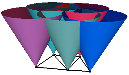
Voronoi Visualization
- Draw a cone in z-direction at each sample \(\vec{p}_i\)
- z-values measure distance from samples, i.e. \(z_i(\vec{x}) = dist(\vec{p}_i,\vec{x})\)
- View cones from below (parallel projection)
- Cone intersections project to Voronoi edges!
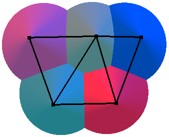
Delaunay Triangulation
- The dual graph of the Voronoi diagram is a planar straight line graph, the Delaunay triangulation (DT)
- Circumcircles of DT triangles are empty
- DT triangles are duals of VD vertices
- Criterion can be used for DT construction
Delaunay Edge Flipping
- Check whether an edge is Delaunay by testing circumcircles of its incident triangles
- Simply flip edge to make it Delaunay!


In-Circle Test
- How to efficiently compute \(\func{InCircle}\of{ \vec{A}, \vec{B}, \vec{C}, \vec{D} }\)?
- Project onto paraboloid: \((x,y) \mapsto (x, y, x^2 + y^2)\)
- Projected points \(\vec{A}'\), \(\vec{B}'\), \(\vec{C}'\) define a plane cutting through the paraboloid
- 3D intersection curve projects to 2D circumcircle
- \(\vec{D}\) is in/out circumcircle \(\Leftrightarrow\) \(\vec{D}'\) is below/above plane
- \(\vec{D}'\) below/above plane \(\Leftrightarrow\) \(\func{volume}(\vec{A}',\vec{B}',\vec{C}',\vec{D}') < 0\) or \(>0\)
- \[\func{volume}(\vec{A}',\vec{B}',\vec{C}',\vec{D}') \;=\; \func{det} \matrix{ A_x & A_y & A_x^2 + A_y^2 & 1 \\ B_x & B_y & B_x^2 + B_y^2 & 1 \\ C_x & C_y & C_x^2 + C_y^2 & 1 \\ D_x & D_y & D_x^2 + D_y^2 & 1} \]


In-Circle Test
- How to efficiently compute \(\func{InCircle}\of{ \vec{A}, \vec{B}, \vec{C}, \vec{D} }\)?
- \[\func{InCircle}\of{\vec{A}, \vec{B}, \vec{C}, \vec{D}} \Leftrightarrow \func{det} \matrix{ A_x & A_y & A_x^2 + A_y^2 & 1 \\ B_x & B_y & B_x^2 + B_y^2 & 1 \\ C_x & C_y & C_x^2 + C_y^2 & 1 \\ D_x & D_y & D_x^2 + D_y^2 & 1 } < 0 \]
- Swapping rows in determinants
- \(\func{InCircle}\of{\vec{A}, \vec{B}, \vec{C}, \vec{D}} == \func{InCircle}\of{\vec{C}, \vec{D}, \vec{A}, \vec{B}}\)
- \(\func{InCircle}\of{\vec{A}, \vec{B}, \vec{C}, \vec{D}} == -\func{InCircle}\of{\vec{B}, \vec{C}, \vec{D}, \vec{A}}\)
![in-circle-test-3.svg]()

Maximum Minimum Angle
- Delaunay criterion maximizes the minimum angle
- Can be seen from Thales’ theorem
![in-circle-test-3.svg]()
- Can be seen from Thales’ theorem
- Delaunay triangulation avoids small angles
- Leads to numerically preferable meshes
- Most important advantage of DT
Incremental Algorithm


Constrained Delaunay Triangulation
- Enforce certain edges in triangulation
- Either prevent flipping (\(\rightarrow\) bad triangles)
- Or subdivide edges sufficiently (\(\rightarrow\) many triangles)


2D Meshing
2D Meshing
- 2D Delaunay triangulation
- Maximizes minimum angle
- Optimal triangulation for given set of vertices
- Why can there still be bad triangles?
Delaunay Refinement
- Delaunay triangulation might contain bad triangles, depending on vertex distribution
- Measure triangle quality by
- circumradius / shortest-edge
- smallest inner angles

Delaunay Refinement
- Insert new vertices to eliminate bad triangles
- Eliminate “bad” triangles by inserting their circumcenter into the triangulation
- Bad triangle will fail the empty-circumcircle test and will therefore be removed


2D Meshing
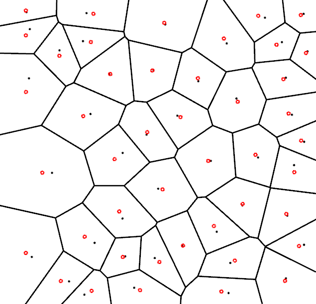
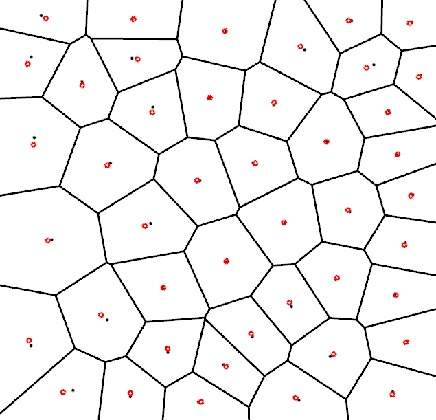
Centroidal Voronoi Diagrams
- How can we get more regular triangulations?
- Delaunay triangulation of Centroidal Voronoi Diagram (CVD)
- Definition:
- All points are centroids of their Voronoi cells
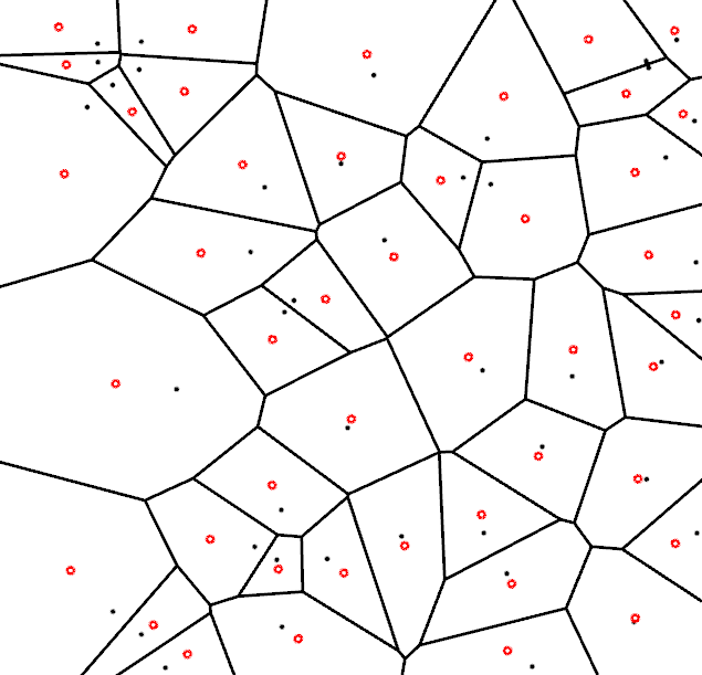
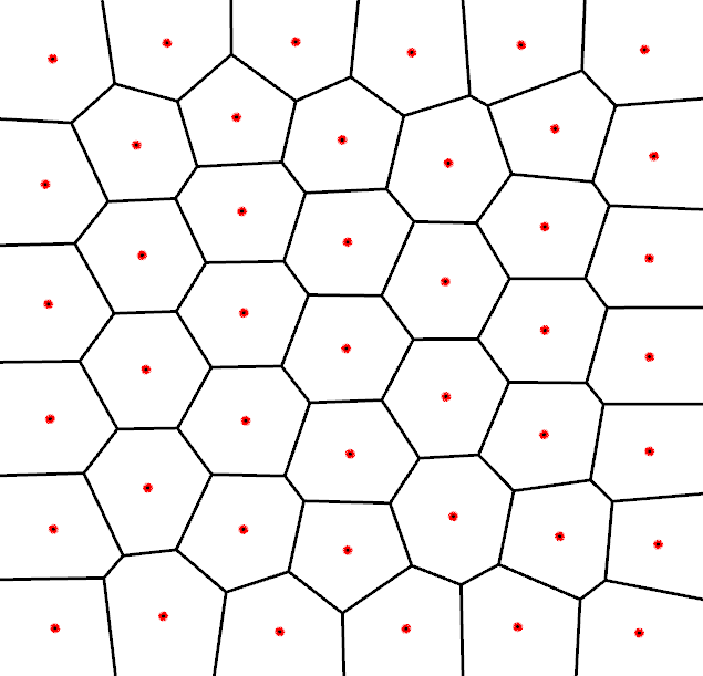
Compute CVD by Lloyd relaxation
- While not converged
- Compute Voronoi diagram of points \(\vec{p}_i\)
- Move \(\vec{p}_i\) to centroids \(\vec{c}_i\) of Voronoi cells \(\set{V}_i\) \[ \vec{p}_i \;\leftarrow\; \vec{c}_i = \left\{ \frac{\int_{\set{V}_i} \vec{x}\cdot\rho(\vec{x}) \func{d}\vec{x}} {\int_{\set{V}_i} \rho(\vec{x}) \func{d}\vec{x}} \right\} \]
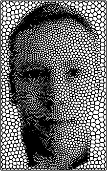
Centroidal Voronoi Diagrams
Literature
- Botsch et al., Polygon Mesh Processing, AK Peters, 2010.
- Chapter 6.4

- de Berg et al., Computational Geometry: Algorithms and Applications, Springer Verlag, 2008.
- O’Rourke, Computational Geometry in C, Cambridge University Press, 1998.