Geometry Processing

Fairing

Edward Chien

Computer Graphics & Geometry Processing

Overview

Recap: Parameterization
Recap: Smoothing
Membrane Surfaces
Thin Plate Surfaces
Linear System Solvers

Parameterization

Discrete Harmonic Maps

Map vertices on boundary \(\partial \set{S}\) homeomorphically to convex polygon \(\bar{\vec{u}}\) in the uv-plane \[\forall v_i \in \partial\set{S} \;:\; \vec{u}\of{v_i} = \bar{\vec{u}}_i\]
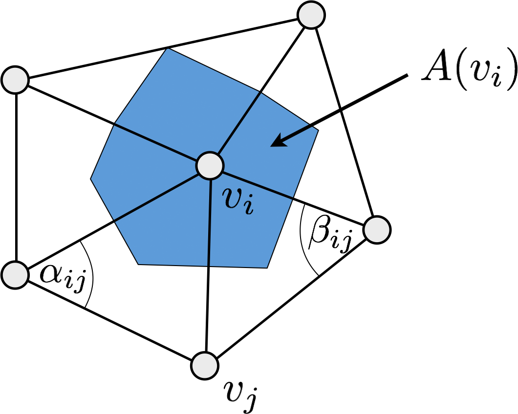
Solve \(\laplace_{\set{S}} \vec{u} = 0\) for all interior vertices \[\forall v_i \in \set{S} \setminus \partial\set{S} \;:\; \sum_{v_j \in \set{N}_1\of{v_i}} \big( \underbrace{\func{cot} \alpha_{ij} + \func{cot} \beta_{ij}}_{w_{ij}} \big) \left( \vec{u}\of{v_j} - \vec{u}\of{v_i} \right) = \vec{0} \]

Iterative Solution

Iterate until convergence
- Solve condition for each interior vertex individually
  (keep weights \(w_{ij}\) fixed) \[ \forall v_i \in \set{S} \setminus \partial\set{S} \;:\; \vec{u}\of{v_i} \;\leftarrow\; \frac{1}{\sum_{v_j \in \set{N}_1\of{v_i}} w_{ij}} \sum_{v_j \in \set{N}_1\of{v_i}} w_{ij} \vec{u}\of{v_j}\]

Why does it converge?
When does it converge?

Direct Solution

Assume that the vertices are partitioned/sorted into interior vertices \(v_1, \dots, v_n\) and boundary vertices \(v_{n+1}, \dots, v_{n+m}\)
Setup \((n+m) \times (n+m)\) system of linear equations from the conditions for interior vertices and boundary vertices \[ \matrix{ \rlap{\laplace_{n \times (n+m)}} \\ \mat{0}_{m \times n} & \mat{I}_{m \times m} } \cdot \matrix{ \vec{u}_1\T \\ \vdots \\ \vec{u}_n\T \\ \vec{u}_{n+1}\T \\ \vdots \\ \vec{u}_{n+m}\T } \;=\; \matrix{ \vec{0}\T \\ \vdots \\ \vec{0}\T \\ \bar{\vec{u}}_{n+1}\T \\ \vdots \\ \bar{\vec{u}}_{n+m}\T } \]

Direct Solution

Simplify this \((n+m) \times (n+m)\) linear system \[ \matrix{ \laplace_{n \times n} & \laplace_{n \times m} \\ \mat{0}_{m \times n} & \mat{I}_{m \times m} } \cdot \matrix{ \vec{u}_1\T \\ \vdots \\ \vec{u}_n\T \\ \vec{u}_{n+1}\T \\ \vdots \\ \vec{u}_{n+m}\T } \;=\; \matrix{ \vec{0}\T \\ \vdots \\ \vec{0}\T \\ \bar{\vec{u}}_{n+1}\T \\ \vdots \\ \bar{\vec{u}}_{n+m}\T } \]
Move the \(m\) known boundary vertices to right hand side
(then we don’t need the bottom \(m\) rows anymore) \[ \laplace_{n \times n} \cdot \matrix{ \vec{u}_1\T \\ \vdots \\ \vec{u}_n\T } \;=\; \matrix{ \vec{0}\T \\ \vdots \\ \vec{0}\T } -\laplace_{n \times m} \matrix{ \bar{\vec{u}}_{n+1}\T \\ \vdots \\ \bar{\vec{u}}_{n+m}\T } \]

Direct Solution

This yields an \(n \times n\) linear system to solve for \(u\) and \(v\) coordinates. \[ \mat{D}\mat{M} \cdot \matrix{ \vec{u}_1\T \\ \vdots \\ \vec{u}_n\T } \;=\; \mat{D}\matrix{ \vec{b}_1\T \\ \vdots \\ \vec{b}_n\T } \]

\[ \begin{align} \mat{M}_{ij} \;&=\; \begin{cases} \func{cot}\alpha_{ij} + \func{cot}\beta_{ij}, & i \ne j \,,\; j \in \set{N}_1\of{v_i} \setminus \partial\set{S} \\ -\sum_{v_j \in \set{N}_1\of{v_i}} \left( \func{cot}\alpha_{ij} + \func{cot}\beta_{ij} \right) & i=j \\ 0 & \text{otherwise} \end{cases} \\[2mm] \mat{D} \;&=\; \func{diag}\of{ \dots, \frac{1}{2A_i}, \dots} \\[2mm] \vec{b}_i \;&=\; -\sum_{v_j \in \set{N}_1\of{v_i} \cap \partial\set{S} } \left( \func{cot}\alpha_{ij} + \func{cot}\beta_{ij} \right) \bar{\vec{u}}_j \end{align} \]

Direct Solution

Let’s make the system symmetric by removing \(\mat{D}\).
And let’s negate it to make the matrix positive definite. \[ -\mat{M} \cdot \matrix{ \vec{u}_1\T \\ \vdots \\ \vec{u}_n\T } \;=\; -\matrix{ \vec{b}_1\T \\ \vdots \\ \vec{b}_n\T } \]

\[ \begin{align} \mat{M}_{ij} \;&=\; \begin{cases} \func{cot}\alpha_{ij} + \func{cot}\beta_{ij}, & i \ne j \,,\; j \in \set{N}_1\of{v_i} \setminus \partial\set{S} \\ -\sum_{v_j \in \set{N}_1\of{v_i}} \left( \func{cot}\alpha_{ij} + \func{cot}\beta_{ij} \right) & i=j \\ 0 & \text{otherwise} \end{cases} \\[2mm] \vec{b}_i \;&=\; -\sum_{v_j \in \set{N}_1\of{v_i} \cap \partial\set{S} } \left( \func{cot}\alpha_{ij} + \func{cot}\beta_{ij} \right) \bar{\vec{u}}_j \end{align} \]

Direct Solution

Solve sparse symmetric positive definite linear system \[ -\mat{M} \cdot \matrix{ \vec{u}_1\T \\ \vdots \\ \vec{u}_n\T } \;=\; -\matrix{ \vec{b}_1\T \\ \vdots \\ \vec{b}_n\T } \]
Allows for efficient linear system solvers
- Iterative: Conjugate Gradients
- Direct: Sparse Cholesky
- more details later…

What about iterative solution?

Iterate until convergence
- Solve condition for each interior vertex individually (keep \(w_{ij}\) fixed) \[ \forall v_i \in \set{S} \setminus \partial\set{S} \;:\; \vec{u}\of{v_i} \;\leftarrow\; \frac{1}{\sum_{v_j \in \set{N}_1\of{v_i}} w_{ij}} \sum_{v_j \in \set{N}_1\of{v_i}} w_{ij} \vec{u}\of{v_j}\]
Why does this work?
- Update corresponds to one Gauss-Seidel iteration for \(\laplace\vec{u}=\vec{0}\).
- When solving \(\mat{A}\vec{x}=\vec{b}\) iterate: \(x_i \leftarrow \frac{1}{a_{ii}} \left( b_i - \sum_{j \neq i} a_{ij} x_j \right)\)
- Solves each condition/row individually, one after the other
- Converges for diagonally dominant matrices: \(\abs{a_{ii}} \geq \sum_{j \neq i} \abs{a_{ij}}\)
- Very simple, but very slow for larger matrices…

Wikipedia: Gauss-Seidel

Try it yourself!

Smoothing

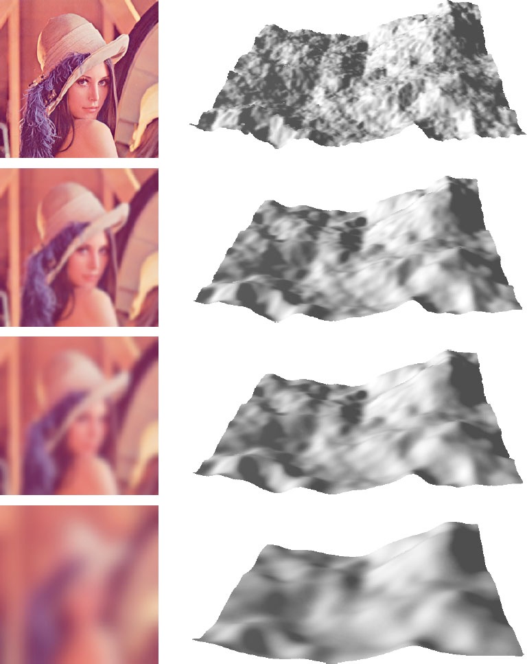
Diffusion Flow

Diffusion equation \[\frac{\partial f}{\partial t} = \lambda \Delta f\]
- \(\lambda\) is the diffusion constant
- \(\Delta\) is the Laplace operator

Wikipedia: Diffusion Equation

Diffusion Flow

2nd order elliptic PDE \[\frac{\partial f(x,y,t)}{\partial t} \;=\; \lambda \left( \frac{\partial^2 f(x,y,t)}{\partial x^2} + \frac{\partial^2 f(x,y,t)}{\partial y^2} \right)\]
Solve numerically
- Discretize in space & time
- Discretize time derivative
- Discretize spatial derivatives

Diffusion Flow in 2D

Diffusion Flow on Meshes

Continuous PDE: \(\frac{\partial \vec{x}}{\partial t} \;=\; \lambda \Delta \vec{x}\)
Discretization: \(\vec{x}_i \leftarrow \vec{x}_i + \delta t \, \lambda \Delta \vec{x}_i\)

Explicit Integration

Use normalized weights and ignore the area term \[\vec{x}_i \leftarrow \vec{x}_i + \delta t \, \lambda \Delta \vec{x}_i\] \[\laplace \vec{x}_i \;=\; \frac{1}{\sum_{v_j \in \set{N}_1\of{v_i}} w_{ij}} \sum_{v_j \in \set{N}_1\of{v_i}} w_{ij} \left( \vec{x}_j - \vec{x}_i \right) \]
Largest stable time-step is \(\delta t \lambda = 1\), which yields \[\vec{x}_i \leftarrow \frac{1}{\sum_{v_j \in \set{N}_1\of{v_i}} w_{ij}} \sum_{v_j \in \set{N}_1\of{v_i}} w_{ij} \vec{x}_j\]
This is exactly one Gauss-Seidel iteration for \(\laplace\vec{x}=0\)!
- Explicit integration will converge to this solution

Implicit Integration

Matrix version of implicit integration \[\left( \mat{I} - \delta t \laplace \right) \, \vec{X}^{(t+1)} = \vec{X}^{(t)}\]
Implicit integration works for any time-step!
Largest stable time-step is \(\infty\), which yields \[ \left( \frac{1}{\delta t}\vec{I} - \laplace \right) \, \vec{X}^{(t+1)} \;=\; \frac{1}{\delta t}\vec{X}^{(t)} \] \[ \underset{\delta t \to \infty}{\longrightarrow} \;\; -\laplace \, \vec{X}^{(t+1)} \;=\; \vec{0} \]
Implicit integration also converges to \(\laplace\vec{x}=\vec{0}\).
- Very similar to parameterization!

Try it yourself!

Fairing

Fair Surfaces

Main idea:
- Penalize “unaesthetic behavior”
- Avoid unnecessary oscillations
- Principle of the simplest shape
Minimize some fairness functional
- Look for physical interpretation
- Minimize surface area → membrane surface
- Minimize curvature → thin plate surface

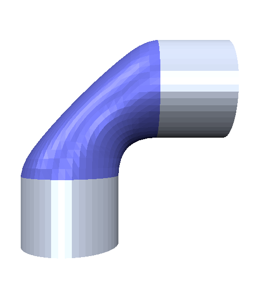
Membrane Surfaces

Minimize surface area \[\int_\set{S} \func{d}A \;\to\; \min \quad\text{with}\quad \delta\set{S}=\bar{\vec{x}}\]
Simpler energy using partial derivatives
(Dirichlet energy) \[\int_\Omega \norm{\vec{x}_{,u}}^2 + \norm{\vec{x}_{,v}}^2 \func{d}u\func{d}v \;\to\;\min\]
Variational calculus gives \[ \begin{align} \laplace_{\set{S}} \vec{x} &= \vec{0}, & \vec{x} \in \set{S} \setminus \partial\set{S} \\ \vec{x} &= \bar{\vec{x}}, & \vec{x} \in \partial\set{S} \end{align} \]

Discretization

Assume that the vertices are partitioned/sorted into interior vertices \(v_1, \dots, v_n\) and boundary vertices \(v_{n+1}, \dots, v_{n+m}\) \[ \matrix{ \rlap{\laplace_{n \times (n+m)}} \\ \mat{0}_{m \times n} & \mat{I}_{m \times m} } \cdot \matrix{ \vec{x}_1\T \\ \vdots \\ \vec{x}_n\T \\ \vec{x}_{n+1}\T \\ \vdots \\ \vec{x}_{n+m}\T } \;=\; \matrix{ \vec{0}\T \\ \vdots \\ \vec{0}\T \\ \bar{\vec{x}}_{n+1}\T \\ \vdots \\ \bar{\vec{x}}_{n+m}\T } \]
Applying same tricks as for parameterization leads to \[ -\mat{M} \cdot \matrix{ \vec{x}_1\T \\ \vdots \\ \vec{x}_n\T } \;=\; -\matrix{ \vec{b}_1\T \\ \vdots \\ \vec{b}_n\T } \]

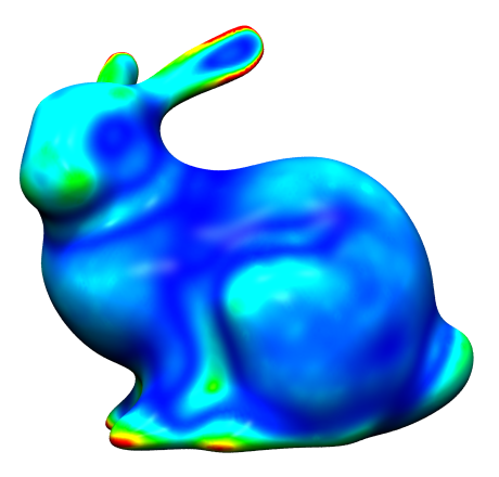
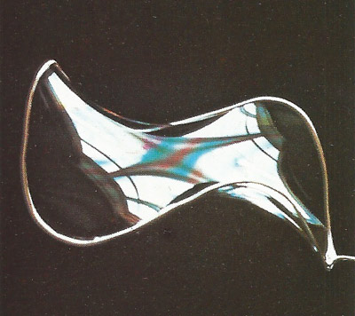
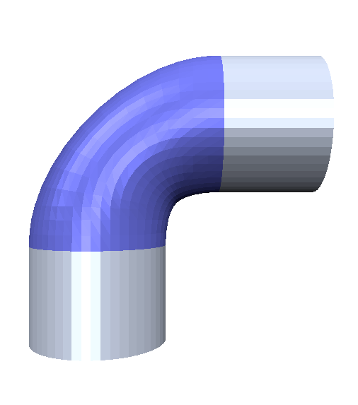
Membrane Surfaces aka Minimal Surface

Mean curvature \(H = \frac{\kappa_1 + \kappa_2}{2}\)
- \(\laplace_{\set{S}} \vec{x} = -2 H \vec{n}\)
- \(H = 0\) everywhere → membrane surface
- \(\laplace_{\set{S}} \vec{x} = \vec{0}\) → smoothing stops

Connection to smoothing & parameterization
- Membrane surfaces are stationary under smoothing
- Smoothing converges to membrane surface
- Parameterization also minimizes area, but flattens boundary first

Wikipedia: Minimal Surface

Try it yourself!

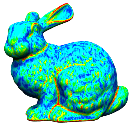
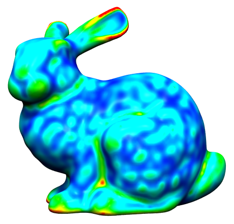
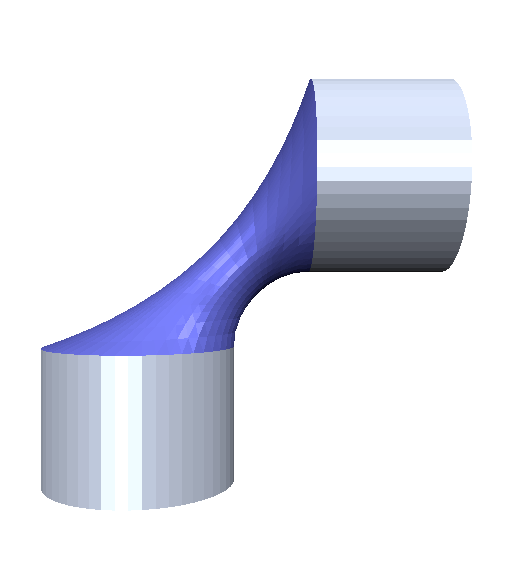
Thin Plate Surfaces

Minimize surface curvature \[\int_\set{S} \kappa_1^2 + \kappa_2^2 \,\func{d}A \to \min \;\text{with}\; \begin{cases} \delta\set{S}=\bar{\vec{x}} \\ \vec{n}\of{\delta\set{S}}=\bar{\vec{n}} \end{cases}\]
Simpler energy using partial derivatives
(thin plate energy) \[\int_\Omega \norm{\vec{x}_{,uu}}^2 + 2\norm{\vec{x}_{,uv}}^2 + \norm{\vec{x}_{,vv}}^2 \func{d}u\func{d}v \;\to\;\min\]
Variational calculus gives \[\begin{align} \laplace_{\set{S}}^2 \vec{x} &= \vec{0}, & \vec{x} \in \set{S} \setminus \partial\set{S} \\ \vec{x} &= \bar{\vec{x}}, & \vec{x} \in \partial\set{S} \\ \vec{n}\of{\vec{x}} &= \bar{\vec{n}}, & \vec{x} \in \partial\set{S} \\ \end{align}\]

Discretization

Assume that the vertices are partitioned into interior vertices \(v_1, \dots, v_n\) and two rings of boundary vertices \(v_{n+1}, \dots, v_{n+m}\) \[ \matrix{ \rlap{\laplace_{n \times (n+m)}^2} \\ \mat{0}_{m \times n} & \mat{I}_{m \times m} } \cdot \matrix{ \vec{x}_1\T \\ \vdots \\ \vec{x}_n\T \\ \vec{x}_{n+1}\T \\ \vdots \\ \vec{x}_{n+m}\T } \;=\; \matrix{ \vec{0}\T \\ \vdots \\ \vec{0}\T \\ \bar{\vec{x}}_{n+1}\T \\ \vdots \\ \bar{\vec{x}}_{n+m}\T } \]
Recursive Laplace discretization \[ \laplace^2 f\of{v_i} \;=\; \laplace\of{\laplace f\of{v_i}} \;=\; \frac{1}{2 A_i} \sum_{v_j \in \set{N}_1\of{v_i}} \left( \func{cot} \alpha_{ij} + \func{cot} \beta_{ij} \right) \left( \laplace f \of{v_j} - \laplace f \of{v_i} \right) \]

Discretization

Assume that the vertices are partitioned into interior vertices \(v_1, \dots, v_n\) and two rings of boundary vertices \(v_{n+1}, \dots, v_{n+m}\) \[ \matrix{ \rlap{\laplace_{n \times (n+m)}^2} \\ \mat{0}_{m \times n} & \mat{I}_{m \times m} } \cdot \matrix{ \vec{x}_1\T \\ \vdots \\ \vec{x}_n\T \\ \vec{x}_{n+1}\T \\ \vdots \\ \vec{x}_{n+m}\T } \;=\; \matrix{ \vec{0}\T \\ \vdots \\ \vec{0}\T \\ \bar{\vec{x}}_{n+1}\T \\ \vdots \\ \bar{\vec{x}}_{n+m}\T } \]
Move fixed vertices to right hand side and remove one \(\mat{D}\) \[ \mat{M}\mat{D}\mat{M} \cdot \matrix{ \vec{x}_1\T \\ \vdots \\ \vec{x}_n\T } \;=\; \matrix{ \vec{b}_1\T \\ \vdots \\ \vec{b}_n\T } \]

Energy Functionals

\[\laplace_{\set{S}} \vec{x} = 0\]

\[\laplace_{\set{S}}^2 \vec{x} = 0\]

\[\laplace_{\set{S}}^3 \vec{x} = 0\]

Try it yourself!

Laplace discretization matters!

Linear System Solvers

Solvers for sparse symmetric positive definite systems?
Dense Cholesky factorization
- Cubic complexity, high memory consumption 👎
Iterative conjugate gradients
- Quadratic complexity, low memory consumption 👍
Multigrid solvers
- Linear complexity, but complicated to use 😟
Sparse Cholesky factorization
- Almost linear complexity and very easy to use! 😍

See Scientific Computing Course Notes

Benchmark: Laplace Systems

10k, 20k, 30k, 40k, 50k
Conjugate Gradients, 1.75, 3.78, 5.96, 7.86, 10.72
Multigrid, 0.89, 1.89, 2.96, 4.05, 5.49
Sparse Cholesky, 0.24, 0.51, 0.84, 1.18, 1.54

Benchmark: Laplace Systems

10k, 20k, 30k, 40k, 50k
Conjugate Gradients, 0.08, 0.21, 0.38, 0.56, 0.98
Multigrid, 0.09, 0.19, 0.27, 0.33, 0.57
Sparse Cholesky, 0.01, 0.03, 0.05, 0.06, 0.1

Benchmark: Laplace² Systems

10k, 20k, 30k, 40k, 50k
Conjugate Gradients, 6.55, 14.54, 25.5, 38.33, 44.09
Multigrid, 1.53, 3.17, 4.89, 6.24, 9.21
Sparse Cholesky, 0.63, 1.4, 2.38, 3.34, 4.52

Benchmark: Laplace² Systems

10k, 20k, 30k, 40k, 50k
Conjugate Gradients, 0.44, 1.5, 5.46, 10.6, 8.95
Multigrid, 0.48, 0.84, 1.23, 1.47, 2.34
Sparse Cholesky, 0.03, 0.08, 0.13, 0.2, 0.26

Literature

Botsch et al., Polygon Mesh Processing, AK Peters, 2010
- Chapter 4: Smoothing & Fairing
- Appendix A: Numerics

Desbrun, Meyer, Schröder, Barr: Implicit Fairing of Irregular Meshes using Diffusion and Curvature Flow, SIGGRAPH 1999
Desbrun, Meyer, Alliez: Intrinsic Parameterizations of Surface Meshes, Eurographics 2002
Jacobson, Tosun, Sorkine, Zorin: Mixed Finite Elements for Variational Surface Modeling, SGP 2010

Title

Overview

Parameterization

Discrete Harmonic Maps

Iterative Solution

Direct Solution

Direct Solution

Direct Solution

Direct Solution

Direct Solution

What about iterative solution?

Try it yourself!

Smoothing

Diffusion Flow

Diffusion Flow

Diffusion Flow in 2D

Diffusion Flow on Meshes

Explicit Integration

Implicit Integration

Try it yourself!

Fairing

Fair Surfaces

Membrane Surfaces

Discretization

Membrane Surfaces aka Minimal Surface

Try it yourself!

Thin Plate Surfaces

Discretization

Discretization

Energy Functionals

Try it yourself!

Laplace discretization matters!

Linear System Solvers

Linear System Solvers

Benchmark: Laplace Systems

Benchmark: Laplace Systems

Benchmark: Laplace2 Systems

Benchmark: Laplace2 Systems

Literature

Benchmark: Laplace² Systems

Benchmark: Laplace² Systems