Title

Digital Geometry Processing
Exercise 6 - Smoothing
Edward Chien, edchien@bu.edu
Computer Graphics & Geometry Processing

Exercise 5 Commentary

In-Circle Test (CORRECTED)

  • How to efficiently compute \(\func{InCircle}\of{ \vec{A}, \vec{B}, \vec{C}, \vec{D} }\)?
    • Project onto paraboloid: \((x,y) \mapsto (x, y, x^2 + y^2)\)
    • Projected points \(\vec{A}'\), \(\vec{B}'\), \(\vec{C}'\) define a plane cutting through the paraboloid
    • 3D intersection curve projects to 2D circumcircle
    • \(\vec{D}\) is in/out circumcircle \(\Leftrightarrow\) \(\vec{D}'\) is below/above plane
    • \(\vec{D}'\) below/above plane \(\Leftrightarrow\) \(\func{volume}(\vec{A}',\vec{B}',\vec{C}',\vec{D}') < 0\) or \(>0\)
    • \[\func{volume}(\vec{A}',\vec{B}',\vec{C}',\vec{D}') \;=\; \func{det} \matrix{ C_x & C_y & C_x^2 + A_y^2 & 1 \\ B_x & B_y & B_x^2 + B_y^2 & 1 \\ A_x & A_y & A_x^2 + A_y^2 & 1 \\ D_x & D_y & D_x^2 + D_y^2 & 1} \]

in-circle-test-1.svg in-circle-test-2.svg

Half-edge pointers review

Exercise 6 Information

Numerical Integration

  • Let’s write the position update in matrix notation
  • Write all points \(\vec{x}_i^{(t)}\) in a large vector/matrix: \[\vec{X}^{(t)} = \trans{\left( \vec{x}_1^{(t)}, \ldots, \vec{x}_n^{(t)} \right)} \in \R^{n\times 3}\]
  • Matrix version of explicit integration (requires small \(\delta t \lambda\)) \[\vec{X}^{(t+1)} = (\vec{I} + \delta t \, \lambda \vec{L}) \, \vec{X}^{(t)}\]
  • Matrix version of implicit integration (works for any \(\delta t \lambda\)) \[(\vec{I} - \delta t \, \lambda \vec{L}) \, \vec{X}^{(t+1)} = \vec{X}^{(t)}\]

Wikipedia: Explicit/Implicit Integration

How to solve the linear system?

  • Solve linear system in each iteration \[(\vec{I} - \delta t \, \lambda \vec{L}) \vec{X}^{(t+1)} = \vec{X}^{(t)}\]
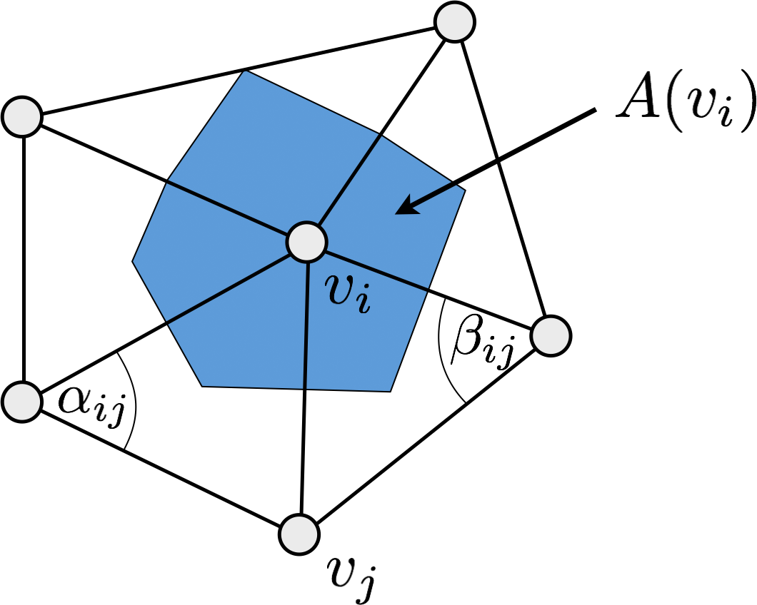
  • Matrix \(\vec{L} = \vec{DM}\) is built from Laplace weights \[\mat{M}_{ij} \;=\; \begin{cases} \func{cot}\alpha_{ij} + \func{cot}\beta_{ij}, & i \ne j \,,\; j \in \set{N}_1\of{v_i} \\ - \sum_{v_j \in \set{N}_1 \of{v_i}}\of{ \func{cot}\alpha_{ij} + \func{cot}\beta_{ij} } & i=j \\ 0 & \text{otherwise} \end{cases} \]

\[\mat{D} = \func{diag}\of{ \dots, \frac{1}{2A_i}, \dots}\]

cotanLaplace.png

How to solve the linear system?

  • Solve linear system in each iteration \[(\vec{I} - \delta t \, \lambda \vec{L}) \vec{X}^{(t+1)} = \vec{X}^{(t)}\]
  • Which solvers do you know?
    • Gaussian elimination? πŸ’£
    • LU factorization? πŸ’£
  • Analyze the properties of your system matrix!
    • very sparse (about 7 non-zeros per row) πŸ˜„
    • but not symmetric 😒

How to solve the linear system?

  • Matrix \(\vec{L} = \vec{DM}\) is not symmetric because of \(\vec{D}\).
    Symmetrize it by multiplying with \(\vec{D}^{-1}\) from the left \[(\vec{D}^{-1} - \delta t \, \lambda \vec{M}) \vec{X}^{(t+1)} = \vec{D}^{-1} \vec{X}^{(t)}\]
  • Now the linear system is
    • sparse πŸ˜„
    • symmetric πŸ˜„
    • positive definite πŸ˜„
  • We can use much more efficient solvers!
    • conjugate gradients 😘
    • sparse Cholesky factorization 😍

See Scientific Computing course notes

Some useful methods

// Curvature.hh included in Smoothing.hh, so may use those for edge and vertex weight calculations
calc_edges_weights();
calc_weights();

// Don't forget to update normals after shifting vertex positions for shading purposes
mesh_.update_normals()

Some useful tips

  • Don’t forget that normalized weights are recommended for explicit smoothing
  • Use sparse linear algebra solvers for the implicit smoothing (review Exercise 1!)
    • SimplicialLDLT for Sparse Cholesky
    • ConjugateGradient for an iterative approach
  • Use explicit smoothing for the feature enhancement step