Title
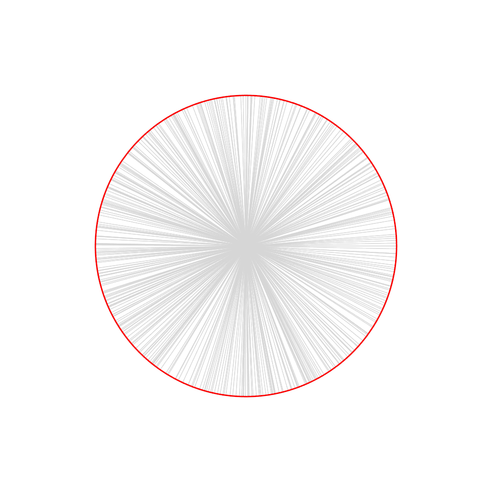
Boundary Initialization
- Map the boundary vertices to a circle with \(\_radius\) in the XY plane


Results
- Texture after 50 iterations with iterative solver
Direct Solution
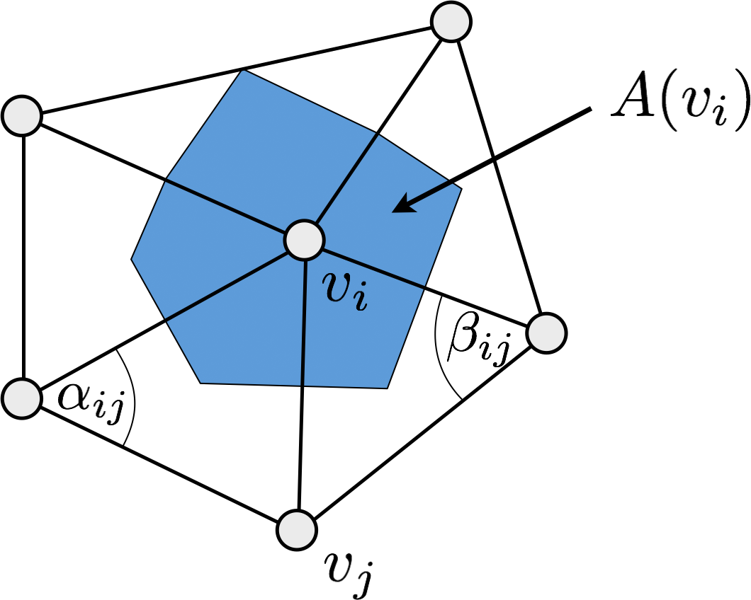
- This yields an \(n \times n\) linear system to solve for \(u\) and \(v\) coordinates. \[ \mat{D}\mat{M} \cdot \matrix{ \vec{u}_1\T \\ \vdots \\ \vec{u}_n\T } \;=\; \mat{D}\matrix{ \vec{b}_1\T \\ \vdots \\ \vec{b}_n\T } \]
\[ \begin{align} \mat{M}_{ij} \;&=\; \begin{cases} \func{cot}\alpha_{ij} + \func{cot}\beta_{ij}, & i \ne j \,,\; j \in \set{N}_1\of{v_i} \setminus \partial\set{S} \\ -\sum_{v_j \in \set{N}_1\of{v_i}} \left( \func{cot}\alpha_{ij} + \func{cot}\beta_{ij} \right) & i=j \\ 0 & \text{otherwise} \end{cases} \\[2mm] \mat{D} \;&=\; \func{diag}\of{ \dots, \frac{1}{2A_i}, \dots} \\[2mm] \vec{b}_i \;&=\; -\sum_{v_j \in \set{N}_1\of{v_i} \cap \partial\set{S} } \left( \func{cot}\alpha_{ij} + \func{cot}\beta_{ij} \right) \bar{\vec{u}}_j \end{align} \]
Direct Solution
- Let’s make the system symmetric by removing \(\mat{D}\).
And let’s negate it to make the matrix positive definite. \[ -\mat{M} \cdot \matrix{ \vec{u}_1\T \\ \vdots \\ \vec{u}_n\T } \;=\; -\matrix{ \vec{b}_1\T \\ \vdots \\ \vec{b}_n\T } \]
\[ \begin{align} \mat{M}_{ij} \;&=\; \begin{cases} \func{cot}\alpha_{ij} + \func{cot}\beta_{ij}, & i \ne j \,,\; j \in \set{N}_1\of{v_i} \setminus \partial\set{S} \\ -\sum_{v_j \in \set{N}_1\of{v_i}} \left( \func{cot}\alpha_{ij} + \func{cot}\beta_{ij} \right) & i=j \\ 0 & \text{otherwise} \end{cases} \\[2mm] \vec{b}_i \;&=\; -\sum_{v_j \in \set{N}_1\of{v_i} \cap \partial\set{S} } \left( \func{cot}\alpha_{ij} + \func{cot}\beta_{ij} \right) \bar{\vec{u}}_j \end{align} \]
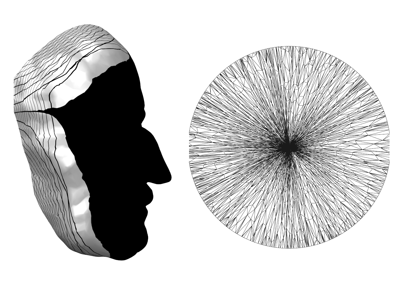
Results
- The result of direct solver

Results
- The initial cylinder1 model and its minimal surface variant when keeping the lower and upper circle boundaries fixed
